Model predictive control python toolbox

do-mpc is a comprehensive open-source toolbox for robust model predictive control (MPC) and moving horizon estimation (MHE). do-mpc enables the efficient formulation and solution of control and estimation problems for nonlinear systems, including tools to deal with uncertainty and time discretization. The modular structure of do-mpc contains simulation, estimation and control components that can be easily extended and combined to fit many different applications.

In summary, do-mpc offers the following features:

• nonlinear and economic model predictive control
• robust multi-stage model predictive control
• moving horizon state and parameter estimation
• modular design that can be easily extended

The do-mpc software is Python based and works therefore on any OS with a Python 3.x distribution. do-mpc has been developed by Sergio Lucia and Alexandru Tatulea at the DYN chair of the TU Dortmund lead by Sebastian Engell. The development is continued at the IOT chair of the TU Berlin by Felix Fiedler and Sergio Lucia.

Example: Robust Multi-stage MPC

We showcase an example, where the control task is to regulate the rotating triple-mass-spring system as shown below:

Once excited, the uncontrolled system takes a long time to come to a rest. To influence the system, two stepper motors are connected to the outermost discs via springs. The designed controller will result in something like this:

Assume, we have modeled the system from first principles and identified the parameters in an experiment. We are especially unsure about the exact value of the inertia of the masses. With Multi-stage MPC, we can define different scenarios e.g. \(\pm 10\%\) for each mass and predict as well as optimize multiple state and input trajectories. This family of trajectories will always obey to set constraints for states and inputs and can be visualized as shown below:

Next steps

We suggest you start by skimming over the selected examples below to get an first impression of the above mentioned features. A great further read for interested viewers is the getting started: MPC page, where we show how to setup do-mpc for the robust control task of a triple-mass-spring system. A state and parameter moving horizon estimator is configured and used for the same system in getting started: MHE.

To install do-mpc please see our installation instructions.

Table of contents

Getting started: MPC

In this Jupyter Notebook we illustrate the core functionalities of do-mpc.

Open an interactive online Jupyter Notebook with this content on Binder:

We start by importing the required modules, most notably do_mpc.

import numpy as np

# Add do_mpc to path. This is not necessary if it was installed via pip.
import sys
sys.path.append('../../')

# Import do_mpc package:
import do_mpc

One of the essential paradigms of do-mpc is a modular architecture, where individual building bricks can be used independently our jointly, depending on the application.

In the following we will present the configuration, setup and connection between these blocks, starting with the model.

Example system

First, we introduce a simple system for which we setup do-mpc. We want to control a triple mass spring system as depicted below:

Three rotating discs are connected via springs and we denote their angles as \(\phi_1, \phi_2, \phi_3\). The two outermost discs are each connected to a stepper motor with additional springs. The stepper motor angles (\(\phi_{m,1}\) and \(\phi_{m,2}\) are used as inputs to the system. Relevant parameters of the system are the inertia \(\Theta\) of the three discs, the spring constants \(c\) as well as the damping factors \(d\).

The second degree ODE of this system can be written as follows:

\begin{align} \Theta_1 \ddot{\phi}_1 &= -c_1 \left(\phi_1 - \phi_{m,1} \right) -c_2 \left(\phi_1 - \phi_2 \right)- d_1 \dot{\phi}_1\\ \Theta_2 \ddot{\phi}_2 &= -c_2 \left(\phi_2 - \phi_{1} \right) -c_3 \left(\phi_2 - \phi_3 \right)- d_2 \dot{\phi}_2\\ \Theta_3 \ddot{\phi}_3 &= -c_3 \left(\phi_3 - \phi_2 \right) -c_4 \left(\phi_3 - \phi_{m,2} \right)- d_3 \dot{\phi}_3 \end{align}

The uncontrolled system, starting from a non-zero initial state will osciallate for an extended period of time, as shown below:

Later, we want to be able to use the motors efficiently to bring the oscillating masses to a rest. It will look something like this:

Creating the model

As indicated above, the model block is essential for the application of do-mpc. In mathmatical terms the model is defined either as a continuous ordinary differential equation (ODE), a differential algebraic equation (DAE) or a discrete equation).

In the case of an DAE/ODE we write:

\begin{align} \frac{\partial x}{\partial t} &= f(x,u,z,p)\\ 0 &= g(x,u,z,p)\\ y &= h(x,u,z,p) \end{align}

We denote \(x\in \mathbb{R}^{n_x}\) as the states, \(u \in \mathbb{R}^{n_u}\) as the inputs, \(z\in \mathbb{R}^{n_z}\) the algebraic states and \(p \in \mathbb{R}^{n_p}\) as parameters.

We reformulate the second order ODEs above as the following first order ODEs, be introducing the following states:

\begin{align} x_1 &= \phi_1\\ x_2 &= \phi_2\\ x_3 &= \phi_3\\ x_4 &= \dot{\phi}_1\\ x_5 &= \dot{\phi}_2\\ x_6 &= \dot{\phi}_3\\ \end{align}

and derive the right-hand-side function \(f(x,u,z,p)\) as:

\begin{align} \dot{x}_1 &= x_4\\ \dot{x}_2 &= x_5\\ \dot{x}_3 &= x_6\\ \dot{x}_4 &= -\frac{c_1}{\Theta_1} \left(x_1 - u_1 \right) -\frac{c_2}{\Theta_1} \left(x1 - x_2 \right)- \frac{d_1}{\Theta_1} x_4\\ \dot{x}_5 &= -\frac{c_2}{\Theta_2} \left(x_2 - x_1 \right) -\frac{c_3}{\Theta_2} \left(x_2 - x_3 \right)- \frac{d_2}{\Theta_2} x_5\\ \dot{x}_6 &= -\frac{c_3}{\Theta_3} \left(x_3 - x_2 \right) -\frac{c_4}{\Theta_3} \left(x_4 - u_2 \right)- \frac{d_3}{\Theta_3} x_6\\ \end{align}

With this theoretical background we can start configuring the do-mpc model object.

First, we need to decide on the model type. For the given example, we are working with a continuous model.

model_type = 'continuous' # either 'discrete' or 'continuous'
model = do_mpc.model.Model(model_type)

Model variables

The next step is to define the model variables. It is important to define the variable type, name and optionally shape (default is scalar variable). The following types are available:

Long name	short name	Remark
states	_x	Required
inputs	_u	Required
algebraic	_z	Optional
parameter	_p	Optional
timevarying_parameter	_tvp	Optional

phi_1 = model.set_variable(var_type='_x', var_name='phi_1', shape=(1,1))
phi_2 = model.set_variable(var_type='_x', var_name='phi_2', shape=(1,1))
phi_3 = model.set_variable(var_type='_x', var_name='phi_3', shape=(1,1))
# Variables can also be vectors:
dphi = model.set_variable(var_type='_x', var_name='dphi', shape=(3,1))
# Two states for the desired (set) motor position:
phi_m_1_set = model.set_variable(var_type='_u', var_name='phi_m_1_set')
phi_m_2_set = model.set_variable(var_type='_u', var_name='phi_m_2_set')
# Two additional states for the true motor position:
phi_1_m = model.set_variable(var_type='_x', var_name='phi_1_m', shape=(1,1))
phi_2_m = model.set_variable(var_type='_x', var_name='phi_2_m', shape=(1,1))

Note that model.set_variable() returns the symbolic variable:

print('phi_1={}, with phi_1.shape={}'.format(phi_1, phi_1.shape))
print('dphi={}, with dphi.shape={}'.format(dphi, dphi.shape))

phi_1=phi_1, with phi_1.shape=(1, 1)
dphi=[dphi_0, dphi_1, dphi_2], with dphi.shape=(3, 1)

Query variables

If at any time you need to obtain the model variables, e.g. if you create the model in a different file than additional do-mpc modules, you might need to retrieve the defined variables. do-mpc facilitates this process with the Model properties x, u, z, p, tvp, y and aux:

model.x

<casadi.tools.structure3.ssymStruct at 0x7fa718a27d30>

The properties itself a structured symbolic variables, which hold the user-defined variables. These can be accessed with indices:

model.x['phi_1']

SX(phi_1)

Note that this is identical to the output of model.set_variable from above:

bool(model.x['phi_1'] == phi_1)

True

Further indices are possible in the case of variables with multiple elements:

model.x['dphi',0]

SX(dphi_0)

Note that you can use the following methods:

• .keys()
• .labels()

to get more information from the symbolic structures:

model.x.keys()

['phi_1', 'phi_2', 'phi_3', 'dphi', 'phi_1_m', 'phi_2_m']

model.x.labels()

['[phi_1,0]',
 '[phi_2,0]',
 '[phi_3,0]',
 '[dphi,0]',
 '[dphi,1]',
 '[dphi,2]',
 '[phi_1_m,0]',
 '[phi_2_m,0]']

Model parameters

Next we define parameters. Known values can and should be hardcoded but with robust MPC in mind, we define uncertain parameters explictly. We assume that the inertia is such an uncertain parameter and hardcode the spring constant and friction coefficient.

# As shown in the table above, we can use Long names or short names for the variable type.
Theta_1 = model.set_variable('parameter', 'Theta_1')
Theta_2 = model.set_variable('parameter', 'Theta_2')
Theta_3 = model.set_variable('parameter', 'Theta_3')

c = np.array([2.697,  2.66,  3.05, 2.86])*1e-3
d = np.array([6.78,  8.01,  8.82])*1e-5

Right-hand-side equation

Finally, we set the right-hand-side of the model by calling model.set_rhs(var_name, expr) with the var_name from the state variables defined above and an expression in terms of \(x, u, z, p\).

model.set_rhs('phi_1', dphi[0])
model.set_rhs('phi_2', dphi[1])
model.set_rhs('phi_3', dphi[2])

For the vector valued state dphi we need to concatenate symbolic expressions. We import the symbolic library CasADi:

from casadi import *

dphi_next = vertcat(
    -c[0]/Theta_1*(phi_1-phi_1_m)-c[1]/Theta_1*(phi_1-phi_2)-d[0]/Theta_1*dphi[0],
    -c[1]/Theta_2*(phi_2-phi_1)-c[2]/Theta_2*(phi_2-phi_3)-d[1]/Theta_2*dphi[1],
    -c[2]/Theta_3*(phi_3-phi_2)-c[3]/Theta_3*(phi_3-phi_2_m)-d[2]/Theta_3*dphi[2],
)

model.set_rhs('dphi', dphi_next)

tau = 1e-2
model.set_rhs('phi_1_m', 1/tau*(phi_m_1_set - phi_1_m))
model.set_rhs('phi_2_m', 1/tau*(phi_m_2_set - phi_2_m))

The model setup is completed by calling model.setup():

model.setup()

After calling model.setup() we cannot define further variables etc.

Configuring the MPC controller

With the configured and setup model we can now create the optimizer for model predictive control (MPC). We start by creating the object (with the model as the only input)

mpc = do_mpc.controller.MPC(model)

Optimizer parameters

Next, we need to parametrize the optimizer. Please see the API documentation for optimizer.set_param() for a full description of available parameters and their meaning. Many parameters already have suggested default values. Most importantly, we need to set n_horizon and t_step. We also choose n_robust=1 for this example, which would default to 0.

Note that by default the continuous system is discretized with collocation.

setup_mpc = {
    'n_horizon': 20,
    't_step': 0.1,
    'n_robust': 1,
    'store_full_solution': True,
}
mpc.set_param(**setup_mpc)

Objective function

The MPC formulation is at its core an optimization problem for which we need to define an objective function:

\[C = \sum_{k=0}^{n-1}\left( \underbrace{l(x_k,u_k,z_k,p)}_{\text{lagrange term}} + \underbrace{\Delta u_k^T R \Delta u_k}_{\text{r-term}}\right) + \underbrace{m(x_n)}_{\text{meyer term}}\]

We need to define the meyer term (mterm) and lagrange term (lterm). For the given example we set:

\[\begin{split}l(x_k,u_k,z_k,p) = \phi_1^2+\phi_2^2+\phi_3^2\\ m(x_n) = \phi_1^2+\phi_2^2+\phi_3^2\end{split}\]

mterm = phi_1**2 + phi_2**2 + phi_3**2
lterm = phi_1**2 + phi_2**2 + phi_3**2

mpc.set_objective(mterm=mterm, lterm=lterm)

Part of the objective function is also the penality for the control inputs. This penalty can often be used to smoothen the obtained optimal solution and is an important tuning parameter. We add a quadratic penalty on changes:

\[\Delta u_k = u_k - u_{k-1}\]

and automatically supply the solver with the previous solution of \(u_{k-1}\) for \(\Delta u_0\).

The user can set the tuning factor for these quadratic terms like this:

mpc.set_rterm(
    phi_m_1_set=1e-2,
    phi_m_2_set=1e-2
)

where the keyword arguments refer to the previously defined input names. Note that in the notation above (\(\Delta u_k^T R \Delta u_k\)), this results in setting the diagonal elements of \(R\).

Constraints

It is an important feature of MPC to be able to set constraints on inputs and states. In do-mpc these constraints are set like this:

# Lower bounds on states:
mpc.bounds['lower','_x', 'phi_1'] = -2*np.pi
mpc.bounds['lower','_x', 'phi_2'] = -2*np.pi
mpc.bounds['lower','_x', 'phi_3'] = -2*np.pi
# Upper bounds on states
mpc.bounds['upper','_x', 'phi_1'] = 2*np.pi
mpc.bounds['upper','_x', 'phi_2'] = 2*np.pi
mpc.bounds['upper','_x', 'phi_3'] = 2*np.pi

# Lower bounds on inputs:
mpc.bounds['lower','_u', 'phi_m_1_set'] = -2*np.pi
mpc.bounds['lower','_u', 'phi_m_2_set'] = -2*np.pi
# Lower bounds on inputs:
mpc.bounds['upper','_u', 'phi_m_1_set'] = 2*np.pi
mpc.bounds['upper','_u', 'phi_m_2_set'] = 2*np.pi

Scaling

Scaling is an important feature if the OCP is poorly conditioned, e.g. different states have significantly different magnitudes. In that case the unscaled problem might not lead to a (desired) solution. Scaling factors can be introduced for all states, inputs and algebraic variables and the objective is to scale them to roughly the same order of magnitude. For the given problem, this is not necessary but we briefly show the syntax (note that this step can also be skipped).

mpc.scaling['_x', 'phi_1'] = 2
mpc.scaling['_x', 'phi_2'] = 2
mpc.scaling['_x', 'phi_3'] = 2

Uncertain Parameters

An important feature of do-mpc is scenario based robust MPC. Instead of predicting and controlling a single future trajectory, we investigate multiple possible trajectories depending on different uncertain parameters. These parameters were previously defined in the model (the mass inertia). Now we must provide the optimizer with different possible scenarios.

This can be done in the following way:

inertia_mass_1 = 2.25*1e-4*np.array([1., 0.9, 1.1])
inertia_mass_2 = 2.25*1e-4*np.array([1., 0.9, 1.1])
inertia_mass_3 = 2.25*1e-4*np.array([1.])

mpc.set_uncertainty_values(
    Theta_1 = inertia_mass_1,
    Theta_2 = inertia_mass_2,
    Theta_3 = inertia_mass_3
)

We provide a number of keyword arguments to the method optimizer.set_uncertain_parameter(). For each referenced parameter the value is a numpy.ndarray with a selection of possible values. The first value is the nominal case, where further values will lead to an increasing number of scenarios. Since we investigate each combination of possible parameters, the number of scenarios is growing rapidly. For our example, we are therefore only treating the inertia of mass 1 and 2 as uncertain and supply only one possible value for the mass of inertia 3.

Setup

The last step of configuring the optimizer is to call optimizer.setup, which finalizes the setup and creates the optimization problem. Only now can we use the optimizer to obtain the control input.

mpc.setup()

Configuring the Simulator

In many cases a developed control approach is first tested on a simulated system. do-mpc responds to this need with the do_mpc.simulator class. The simulator uses state-of-the-art DAE solvers, e.g. Sundials CVODE to solve the DAE equations defined in the supplied do_mpc.model. This will often be the same model as defined for the optimizer but it is also possible to use a more complex model of the same system.

In this section we demonstrate how to setup the simulator class for the given example. We initilize the class with the previously defined model:

simulator = do_mpc.simulator.Simulator(model)

Simulator parameters

Next, we need to parametrize the simulator. Please see the API documentation for simulator.set_param() for a full description of available parameters and their meaning. Many parameters already have suggested default values. Most importantly, we need to set t_step. We choose the same value as for the optimizer.

# Instead of supplying a dict with the splat operator (**), as with the optimizer.set_param(),
# we can also use keywords (and call the method multiple times, if necessary):
simulator.set_param(t_step = 0.1)

Uncertain parameters

In the model we have defined the inertia of the masses as parameters, for which we have chosen multiple scenarios in the optimizer. The simulator is now parametrized to simulate with the “true” values at each timestep. In the most general case, these values can change, which is why we need to supply a function that can be evaluted at each time to obtain the current values. do-mpc requires this function to have a specific return structure which we obtain first by calling:

p_template = simulator.get_p_template()

This object is a CasADi structure:

type(p_template)

casadi.tools.structure3.DMStruct

which can be indexed with the following keys:

p_template.keys()

['default', 'Theta_1', 'Theta_2', 'Theta_3']

We need to now write a function which returns this structure with the desired numerical values. For our simple case:

def p_fun(t_now):
    p_template['Theta_1'] = 2.25e-4
    p_template['Theta_2'] = 2.25e-4
    p_template['Theta_3'] = 2.25e-4
    return p_template

This function is now supplied to the simulator in the following way:

simulator.set_p_fun(p_fun)

Setup

Similarly to the optimizer we need to call simulator.setup() to finalize the setup of the simulator.

simulator.setup()

Creating the control loop

In theory, we could now also create an estimator but for this concise example we just assume direct state-feedback. This means we are now ready to setup and run the control loop. The control loop consists of running the optimizer with the current state (\(x_0\)) to obtain the current control input (\(u_0\)) and then running the simulator with the current control input (\(u_0\)) to obtain the next state.

As discussed before, we setup a controller for regulating a triple-mass-spring system. To show some interesting control action we choose an arbitrary initial state \(x_0\neq 0\):

x0 = np.pi*np.array([1, 1, -1.5, 1, -1, 1, 0, 0]).reshape(-1,1)

and use the x0 property to set the initial state.

simulator.x0 = x0
mpc.x0 = x0

While we are able to set just a regular numpy array, this populates the state structure which was inherited from the model:

mpc.x0

<casadi.tools.structure3.DMStruct at 0x7fa71b5ee390>

We can thus easily obtain the value of particular states by calling:

mpc.x0['phi_1']

DM(3.14159)

Note that the properties x0 (as well as u0, z0 and t0) always display the values of the current variables in the class.

To set the initial guess of the MPC optimization problem we call:

mpc.set_initial_guess()

The chosen initial guess is based on x0, z0 and u0 which are set for each element of the MPC sequence.

Setting up the Graphic

To investigate the controller performance AND the MPC predictions, we are using the do-mpc graphics module. This versatile tool allows us to conveniently configure a user-defined plot based on Matplotlib and visualize the results stored in the mpc.data, simulator.data (and if applicable estimator.data) objects.

We start by importing matplotlib:

import matplotlib.pyplot as plt
import matplotlib as mpl
# Customizing Matplotlib:
mpl.rcParams['font.size'] = 18
mpl.rcParams['lines.linewidth'] = 3
mpl.rcParams['axes.grid'] = True

And initializing the graphics module with the data object of interest. In this particular example, we want to visualize both the mpc.data as well as the simulator.data.

mpc_graphics = do_mpc.graphics.Graphics(mpc.data)
sim_graphics = do_mpc.graphics.Graphics(simulator.data)

Next, we create a figure and obtain its axis object. Matplotlib offers multiple alternative ways to obtain an axis object, e.g. subplots, subplot2grid, or simply gca. We use subplots:

%%capture
# We just want to create the plot and not show it right now. This "inline magic" supresses the output.
fig, ax = plt.subplots(2, sharex=True, figsize=(16,9))
fig.align_ylabels()

Most important API element for setting up the graphics module is graphics.add_line, which mimics the API of model.add_variable, except that we also need to pass an axis.

We want to show both the simulator and MPC results on the same axis, which is why we configure both of them identically:

%%capture
for g in [sim_graphics, mpc_graphics]:
    # Plot the angle positions (phi_1, phi_2, phi_2) on the first axis:
    g.add_line(var_type='_x', var_name='phi_1', axis=ax[0])
    g.add_line(var_type='_x', var_name='phi_2', axis=ax[0])
    g.add_line(var_type='_x', var_name='phi_3', axis=ax[0])

    # Plot the set motor positions (phi_m_1_set, phi_m_2_set) on the second axis:
    g.add_line(var_type='_u', var_name='phi_m_1_set', axis=ax[1])
    g.add_line(var_type='_u', var_name='phi_m_2_set', axis=ax[1])


ax[0].set_ylabel('angle position [rad]')
ax[1].set_ylabel('motor angle [rad]')
ax[1].set_xlabel('time [s]')

Running the simulator

We start investigating the do-mpc simulator and the graphics package by simulating the autonomous system without control inputs (\(u = 0\)). This can be done as follows:

u0 = np.zeros((2,1))
for i in range(200):
    simulator.make_step(u0)

We can visualize the resulting trajectory with the pre-defined graphic:

sim_graphics.plot_results()
# Reset the limits on all axes in graphic to show the data.
sim_graphics.reset_axes()
# Show the figure:
fig

As desired, the motor angle (input) is constant at zero and the oscillating masses slowly come to a rest. Our control goal is to significantly shorten the time until the discs are stationary.

Remember the animation you saw above, of the uncontrolled system? This is where the data came from.

Running the optimizer

To obtain the current control input we call optimizer.make_step(x0) with the current state (\(x_0\)):

u0 = mpc.make_step(x0)

******************************************************************************
This program contains Ipopt, a library for large-scale nonlinear optimization.
 Ipopt is released as open source code under the Eclipse Public License (EPL).
         For more information visit http://projects.coin-or.org/Ipopt
******************************************************************************

This is Ipopt version 3.12.3, running with linear solver mumps.
NOTE: Other linear solvers might be more efficient (see Ipopt documentation).

Number of nonzeros in equality constraint Jacobian...:    19448
Number of nonzeros in inequality constraint Jacobian.:        0
Number of nonzeros in Lagrangian Hessian.............:     1229

Total number of variables............................:     6408
                     variables with only lower bounds:        0
                variables with lower and upper bounds:     2435
                     variables with only upper bounds:        0
Total number of equality constraints.................:     5768
Total number of inequality constraints...............:        0
        inequality constraints with only lower bounds:        0
   inequality constraints with lower and upper bounds:        0
        inequality constraints with only upper bounds:        0

iter    objective    inf_pr   inf_du lg(mu)  ||d||  lg(rg) alpha_du alpha_pr  ls
   0  8.8086219e+02 1.65e+01 1.07e-01  -1.0 0.00e+00    -  0.00e+00 0.00e+00   0
   1  2.8794996e+02 2.32e+00 1.68e+00  -1.0 1.38e+01  -4.0 2.82e-01 8.60e-01f  1
   2  2.0017562e+02 1.87e-14 3.95e+00  -1.0 3.56e+00  -4.5 1.96e-01 1.00e+00f  1
   3  1.6039802e+02 1.48e-14 3.82e-01  -1.0 3.43e+00  -5.0 5.14e-01 1.00e+00f  1
   4  1.3046012e+02 2.04e-14 7.36e-02  -1.0 2.94e+00  -5.4 7.75e-01 1.00e+00f  1
   5  1.1452477e+02 2.04e-14 1.94e-02  -1.7 2.62e+00  -5.9 8.44e-01 1.00e+00f  1
   6  1.1247422e+02 1.87e-14 7.23e-03  -2.5 9.17e-01  -6.4 8.27e-01 1.00e+00f  1
   7  1.1235000e+02 1.69e-14 4.88e-08  -2.5 3.56e-01  -6.9 1.00e+00 1.00e+00f  1
   8  1.1230585e+02 1.87e-14 8.91e-09  -3.8 1.95e-01  -7.3 1.00e+00 1.00e+00f  1
   9  1.1229857e+02 1.83e-14 8.02e-10  -5.7 5.26e-02  -7.8 1.00e+00 1.00e+00f  1
iter    objective    inf_pr   inf_du lg(mu)  ||d||  lg(rg) alpha_du alpha_pr  ls
  10  1.1229833e+02 1.51e-14 6.08e-09  -5.7 1.20e+00  -8.3 1.00e+00 1.00e+00f  1
  11  1.1229831e+02 1.69e-14 3.25e-13  -8.6 1.92e-04  -8.8 1.00e+00 1.00e+00f  1

Number of Iterations....: 11

                                   (scaled)                 (unscaled)
Objective...............:   1.1229831239969913e+02    1.1229831239969913e+02
Dual infeasibility......:   3.2479227640713759e-13    3.2479227640713759e-13
Constraint violation....:   1.6875389974302379e-14    1.6875389974302379e-14
Complementarity.........:   4.2481089749952700e-09    4.2481089749952700e-09
Overall NLP error.......:   4.2481089749952700e-09    4.2481089749952700e-09


Number of objective function evaluations             = 12
Number of objective gradient evaluations             = 12
Number of equality constraint evaluations            = 12
Number of inequality constraint evaluations          = 0
Number of equality constraint Jacobian evaluations   = 12
Number of inequality constraint Jacobian evaluations = 0
Number of Lagrangian Hessian evaluations             = 11
Total CPU secs in IPOPT (w/o function evaluations)   =      0.239
Total CPU secs in NLP function evaluations           =      0.006

EXIT: Optimal Solution Found.
           S  :   t_proc      (avg)   t_wall      (avg)    n_eval
       nlp_f  | 149.00us ( 12.42us) 145.00us ( 12.08us)        12
       nlp_g  |   2.16ms (180.17us)   1.83ms (152.33us)        12
    nlp_grad  | 377.00us (377.00us) 377.00us (377.00us)         1
  nlp_grad_f  | 504.00us ( 38.77us) 525.00us ( 40.38us)        13
  nlp_hess_l  | 138.00us ( 12.55us) 137.00us ( 12.45us)        11
   nlp_jac_g  |   3.27ms (251.31us)   3.26ms (251.00us)        13
       total  | 257.31ms (257.31ms) 256.06ms (256.06ms)         1

Note that we obtained the output from IPOPT regarding the given optimal control problem (OCP). Most importantly we obtained Optimal Solution Found.

We can also visualize the predicted trajectories with the configure graphics instance. First we clear the existing lines from the simulator by calling:

sim_graphics.clear()

And finally, we can call plot_predictions to obtain:

mpc_graphics.plot_predictions()
mpc_graphics.reset_axes()
# Show the figure:
fig

We are seeing the predicted trajectories for the states and the optimal control inputs. Note that we are seeing different scenarios for the configured uncertain inertia of the three masses.

We can also see that the solution is considering the defined upper and lower bounds. This is especially true for the inputs.

Changing the line appearance

Before we continue, we should probably improve the visualization a bit. We can easily obtain all line objects from the graphics module by using the result_lines and pred_lines properties:

mpc_graphics.pred_lines

<do_mpc.tools.structure.Structure at 0x7fa71b5ee860>

We obtain a structure that can be queried conveniently as follows:

mpc_graphics.pred_lines['_x', 'phi_1']

[<matplotlib.lines.Line2D at 0x7fa71c445828>,
 <matplotlib.lines.Line2D at 0x7fa71c6e7898>,
 <matplotlib.lines.Line2D at 0x7fa71c6e7978>,
 <matplotlib.lines.Line2D at 0x7fa71c7023c8>,
 <matplotlib.lines.Line2D at 0x7fa71c7022b0>,
 <matplotlib.lines.Line2D at 0x7fa71c702630>,
 <matplotlib.lines.Line2D at 0x7fa71c702978>,
 <matplotlib.lines.Line2D at 0x7fa71c702d30>,
 <matplotlib.lines.Line2D at 0x7fa71c702c88>]

We obtain all lines for our first state. To change the color we can simply:

# Change the color for the three states:
for line_i in mpc_graphics.pred_lines['_x', 'phi_1']: line_i.set_color('#1f77b4') # orange
for line_i in mpc_graphics.pred_lines['_x', 'phi_2']: line_i.set_color('#ff7f0e') # blue
for line_i in mpc_graphics.pred_lines['_x', 'phi_3']: line_i.set_color('#2ca02c') # green
# Change the color for the two inputs:
for line_i in mpc_graphics.pred_lines['_u', 'phi_m_1_set']: line_i.set_color('#1f77b4')
for line_i in mpc_graphics.pred_lines['_u', 'phi_m_2_set']: line_i.set_color('#ff7f0e')

# Make all predictions transparent:
for line_i in mpc_graphics.pred_lines.full: line_i.set_alpha(0.2)

Note that we can work in the same way with the result_lines property. For example, we can use it to create a legend:

# Get line objects (note sum of lists creates a concatenated list)
lines = sim_graphics.result_lines['_x', 'phi_1']+sim_graphics.result_lines['_x', 'phi_2']+sim_graphics.result_lines['_x', 'phi_3']

ax[0].legend(lines,'123',title='disc')

# also set legend for second subplot:
lines = sim_graphics.result_lines['_u', 'phi_m_1_set']+sim_graphics.result_lines['_u', 'phi_m_2_set']
ax[1].legend(lines,'12',title='motor')

<matplotlib.legend.Legend at 0x7fa71c712eb8>

Running the control loop

Finally, we are now able to run the control loop as discussed above. We obtain the input from the optimizer and then run the simulator.

To make sure we start fresh, we reset the initial state and erase the history:

simulator.set_initial_state(x0, reset_history=True)
mpc.set_initial_state(x0, reset_history=True)

This is the main-loop. We run 20 steps, whic is identical to the prediction horizon. Note that we use “capture” again, to supress the output from IPOPT.

It is usually suggested to display the output as it contains important information about the state of the solver.

%%capture
for i in range(20):
    u0 = mpc.make_step(x0)
    x0 = simulator.make_step(u0)

We can now plot the previously shown prediction from time \(t=0\), as well as the closed-loop trajectory from the simulator:

# Plot predictions from t=0
mpc_graphics.plot_predictions(t_ind=0)
# Plot results until current time
sim_graphics.plot_results()
sim_graphics.reset_axes()
fig

The simulated trajectory with the nominal value of the parameters follows almost exactly the nominal open-loop predictions. The simulted trajectory is bounded from above and below by further uncertain scenarios.

Data processing

Saving and retrieving results

do-mpc results can be stored and retrieved with the methods save_results and load_results from the do_mpc.data module. We start by importing these methods:

from do_mpc.data import save_results, load_results

The method save_results is passed a list of the do-mpc objects that we want to store. In our case, the optimizer and simulator are available and configured.

Note that by default results are stored in the subfolder results under the name results.pkl. Both can be changed and the folder is created if it doesn’t exist already.

save_results([mpc, simulator])

We investigate the content of the newly created folder:

!ls ./results/

results.pkl

Automatically, the save_results call will check if a file with the given name already exists. To avoid overwriting, the method prepends an index. If we save again, the folder contains:

save_results([mpc, simulator])
!ls ./results/

001_results.pkl results.pkl

The pickled results can be loaded manually by writing:

with open(file_name, 'rb') as f:
    results = pickle.load(f)

or by calling load_results with the appropriate file_name (and path). load_results contains simply the code above for more convenience.

results = load_results('./results/results.pkl')

The obtained results is a dictionary with the data objects from the passed do-mpc modules. Such that: results['optimizer'] and optimizer.data contain the same information (similarly for simulator and, if applicable, estimator).

Working with data objects

The do_mpc.data.Data objects also hold some very useful properties that you should know about. Most importantly, we can query them with indices, such as:

results['mpc']

<do_mpc.data.MPCData at 0x117c4df50>

x = results['mpc']['_x']
x.shape

(20, 8)

As expected, we have 20 elements (we ran the loop for 20 steps) and 8 states. Further indices allow to get selected states:

phi_1 = results['mpc']['_x','phi_1']

phi_1.shape

(20, 1)

For vector-valued states we can even query:

dphi_1 = results['mpc']['_x','dphi', 0]

dphi_1.shape

(20, 1)

Of course, we could also query inputs etc.

Furthermore, we can easily retrieve the predicted trajectories with the prediction method. The syntax is slightly different: The first argument is a tuple that mimics the indices shown above. The second index is the time instance. With the following call we obtain the prediction of phi_1 at time 0:

phi_1_pred = results['mpc'].prediction(('_x','phi_1'), t_ind=0)

phi_1_pred.shape

(1, 21, 9)

The first dimension shows that this state is a scalar, the second dimension shows the horizon and the third dimension refers to the nine uncertain scenarios that were investigated.

Animating results

Animating MPC results, to compare prediction and closed-loop trajectories, allows for a very meaningful investigation of the obtained results.

do-mpc significantly facilitates this process while working hand in hand with Matplotlib for full customizability. Obtaining publication ready animations is as easy as writing the following short blocks of code:

from matplotlib.animation import FuncAnimation, FFMpegWriter, ImageMagickWriter

def update(t_ind):
    sim_graphics.plot_results(t_ind)
    mpc_graphics.plot_predictions(t_ind)
    mpc_graphics.reset_axes()

The graphics module can also be used without restrictions with loaded do-mpc data. This allows for convenient data post-processing, e.g. in a Jupyter Notebook. We simply would have to initiate the graphics module with the loaded results from above.

anim = FuncAnimation(fig, update, frames=20, repeat=False)
gif_writer = ImageMagickWriter(fps=3)
anim.save('anim.gif', writer=gif_writer)

Below we showcase the resulting gif file (not in real-time):

Thank you, for following through this short example on how to use do-mpc. We hope you find the tool and this documentation useful.

We suggest that you have a look at the API documentation for further details on the presented modules, methods and functions.

We also want to emphasize that we skipped over many details, further functions etc. in this introduction. Please have a look at our more complex examples to get a better impression of the possibilities with do-mpc.

Getting started: MHE

Open an interactive online Jupyter Notebook with this content on Binder:

In this Jupyter Notebook we illustrate application of the do-mpc moving horizon estimation module. Please follow first the general Getting Started guide, as we cover the sample example and skip over some previously explained details.

import numpy as np
from casadi import *

# Add do_mpc to path. This is not necessary if it was installed via pip.
import sys
sys.path.append('../../')

# Import do_mpc package:
import do_mpc

Creating the model

First, we need to decide on the model type. For the given example, we are working with a continuous model.

model_type = 'continuous' # either 'discrete' or 'continuous'
model = do_mpc.model.Model(model_type)

The model is based on the assumption that we have additive process and/or measurement noise:

\begin{align} \dot{x}(t) &= f(x(t),u(t),z(t),p(t),p_{\text{tv}}(t))+w(t), \\ y(t) &= h(x(t),u(t),z(t),p(t),p_{\text{tv}}(t))+v(t), \end{align}

we are free to chose, which states and which measurements experience additive noise.

Model variables

The next step is to define the model variables. It is important to define the variable type, name and optionally shape (default is scalar variable).

In contrast to the previous example, we now use vectors for all variables.

phi = model.set_variable(var_type='_x', var_name='phi', shape=(3,1))
dphi = model.set_variable(var_type='_x', var_name='dphi', shape=(3,1))

# Two states for the desired (set) motor position:
phi_m_set = model.set_variable(var_type='_u', var_name='phi_m_set', shape=(2,1))

# Two additional states for the true motor position:
phi_m = model.set_variable(var_type='_x', var_name='phi_m', shape=(2,1))

Model measurements

This step is essential for the state estimation task: We must define a measurable output. Typically, this is a subset of states (or a transformation thereof) as well as the inputs.

Note that some MHE implementations consider inputs separately.

As mentionned above, we need to define for each measurement if additive noise is present. In our case we assume noisy state measurements (\(\phi\)) but perfect input measurements.

# State measurements
phi_meas = model.set_meas('phi_1_meas', phi, meas_noise=True)

# Input measurements
phi_m_set_meas = model.set_meas('phi_m_set_meas', phi_m_set, meas_noise=False)

Model parameters

Next we define parameters. The MHE allows to estimate parameters as well as states. Note that not all parameters must be estimated (as shown in the MHE setup below). We can also hardcode parameters (such as the spring constants c).

Theta_1 = model.set_variable('parameter', 'Theta_1')
Theta_2 = model.set_variable('parameter', 'Theta_2')
Theta_3 = model.set_variable('parameter', 'Theta_3')

c = np.array([2.697,  2.66,  3.05, 2.86])*1e-3
d = np.array([6.78,  8.01,  8.82])*1e-5

Right-hand-side equation

Finally, we set the right-hand-side of the model by calling model.set_rhs(var_name, expr) with the var_name from the state variables defined above and an expression in terms of \(x, u, z, p\).

Note that we can decide whether the inidividual states experience process noise. In this example we choose that the system model is perfect. This is the default setting, so we don’t need to pass this parameter explictly.

model.set_rhs('phi', dphi)

dphi_next = vertcat(
    -c[0]/Theta_1*(phi[0]-phi_m[0])-c[1]/Theta_1*(phi[0]-phi[1])-d[0]/Theta_1*dphi[0],
    -c[1]/Theta_2*(phi[1]-phi[0])-c[2]/Theta_2*(phi[1]-phi[2])-d[1]/Theta_2*dphi[1],
    -c[2]/Theta_3*(phi[2]-phi[1])-c[3]/Theta_3*(phi[2]-phi_m[1])-d[2]/Theta_3*dphi[2],
)

model.set_rhs('dphi', dphi_next, process_noise = False)

tau = 1e-2
model.set_rhs('phi_m', 1/tau*(phi_m_set - phi_m))

The model setup is completed by calling model.setup_model():

model.setup_model()

After calling model.setup_model() we cannot define further variables etc.

Configuring the moving horizon estimator

The first step of configuring the moving horizon estimator is to call the class with a list of all parameters to be estimated. An empty list (default value) means that no parameters are estimated. The list of estimated parameters must be a subset (or all) of the previously defined parameters.

Note

So why did we define Theta_2 and Theta_3 if we do not estimate them?

In many cases we will use the same model for (robust) control and MHE estimation. In that case it is possible to have some external parameters (e.g. weather prediction) that are uncertain but cannot be estimated.

mhe = do_mpc.estimator.MHE(model, ['Theta_1'])

MHE parameters:

Next, we pass MHE parameters. Most importantly, we need to set the time step and the horizon. We also choose to obtain the measurement from the MHE data object. Alternatively, we are able to set a user defined measurement function that is called at each timestep and returns the N previous measurements for the estimation step.

setup_mhe = {
    't_step': 0.1,
    'n_horizon': 10,
    'store_full_solution': True,
    'meas_from_data': True
}
mhe.set_param(**setup_mhe)

Objective function

The most important step of the configuration is to define the objective function for the MHE problem:

\begin{align} \underset{ \begin{array}{c} \mathbf{x}_{0:N+1}, \mathbf{u}_{0:N}, p,\\ \mathbf{w}_{0:N}, \mathbf{v}_{0:N} \end{array} }{\mathrm{min}} &\frac{1}{2}\|x_0-\tilde{x}_0\|_{P_x}^2+\frac{1}{2}\|p-\tilde{p}\|_{P_p}^2 +\sum_{k=0}^{N-1} \left(\frac{1}{2}\|v_k\|_{P_{v,k}}^2 + \frac{1}{2}\|w_k\|_{P_{w,k}}^2\right),\\ &\left.\begin{aligned} \mathrm{s.t.}\quad x_{k+1} &= f(x_k,u_k,z_k,p,p_{\text{tv},k})+ w_k,\\ y_k &= h(x_k,u_k,z_k,p,p_{\text{tv},k}) + v_k, \\ &g(x_k,u_k,z_k,p_k,p_{\text{tv},k}) \leq 0 \end{aligned}\right\} k=0,\dots, N \end{align}

We typically consider the formulation shown above, where the user has to pass the weighting matrices P_x, P_v, P_p and P_w. In our concrete example, we assume a perfect model without process noise and thus P_w is not required.

We set the objective function with the weighting matrices shown below:

P_v = np.diag(np.array([1,1,1]))
P_x = np.eye(8)
P_p = 10*np.eye(1)

mhe.set_default_objective(P_x, P_v, P_p)

Fixed parameters

If the model contains parameters and if we estimate only a subset of these parameters, it is required to pass a function that returns the value of the remaining parameters at each time step.

Furthermore, this function must return a specific structure, which is first obtained by calling:

p_template_mhe = mhe.get_p_template()

Using this structure, we then formulate the following function for the remaining (not estimated) parameters:

def p_fun_mhe(t_now):
    p_template_mhe['Theta_2'] = 2.25e-4
    p_template_mhe['Theta_3'] = 2.25e-4
    return p_template_mhe

This function is finally passed to the mhe instance:

mhe.set_p_fun(p_fun_mhe)

Bounds

The MHE implementation also supports bounds for states, inputs, parameters which can be set as shown below. For the given example, it is especially important to set realistic bounds on the estimated parameter. Otherwise the MHE solution is a poor fit.

mhe.bounds['lower','_u', 'phi_m_set'] = -2*np.pi
mhe.bounds['upper','_u', 'phi_m_set'] = 2*np.pi

mhe.bounds['lower','_p_est', 'Theta_1'] = 1e-5
mhe.bounds['upper','_p_est', 'Theta_1'] = 1e-3

Setup

Similar to the controller, simulator and model, we finalize the MHE configuration by calling:

mhe.setup()

Configuring the Simulator

In many cases, a developed control approach is first tested on a simulated system. do-mpc responds to this need with the do_mpc.simulator class. The simulator uses state-of-the-art DAE solvers, e.g. Sundials CVODE to solve the DAE equations defined in the supplied do_mpc.model. This will often be the same model as defined for the optimizer but it is also possible to use a more complex model of the same system.

In this section we demonstrate how to setup the simulator class for the given example. We initialize the class with the previously defined model:

simulator = do_mpc.simulator.Simulator(model)

Simulator parameters

Next, we need to parametrize the simulator. Please see the API documentation for simulator.set_param() for a full description of available parameters and their meaning. Many parameters already have suggested default values. Most importantly, we need to set t_step. We choose the same value as for the optimizer.

# Instead of supplying a dict with the splat operator (**), as with the optimizer.set_param(),
# we can also use keywords (and call the method multiple times, if necessary):
simulator.set_param(t_step = 0.1)

Parameters

In the model we have defined the inertia of the masses as parameters. The simulator is now parametrized to simulate using the “true” values at each timestep. In the most general case, these values can change, which is why we need to supply a function that can be evaluted at each time to obtain the current values. do-mpc requires this function to have a specific return structure which we obtain first by calling:

p_template_sim = simulator.get_p_template()

We need to define a function which returns this structure with the desired numerical values. For our simple case:

def p_fun_sim(t_now):
    p_template_sim['Theta_1'] = 2.25e-4
    p_template_sim['Theta_2'] = 2.25e-4
    p_template_sim['Theta_3'] = 2.25e-4
    return p_template_sim

This function is now supplied to the simulator in the following way:

simulator.set_p_fun(p_fun_sim)

Setup

Finally, we call:

simulator.setup()

Creating the loop

While the full loop should also include a controller, we are currently only interested in showcasing the estimator. We therefore estimate the states for an arbitrary initial condition and some random control inputs (shown below).

x0 = np.pi*np.array([1, 1, -1.5, 1, -5, 5, 0, 0]).reshape(-1,1)

To make things more interesting we pass the estimator a perturbed initial state:

x0_mhe = x0*(1+0.5*np.random.randn(8,1))

and use the x0 property of the simulator and estimator to set the initial state:

simulator.x0 = x0
mhe.x0_mhe = x0_mhe
mhe.p_est0 = 1e-4

It is also adviced to create an initial guess for the MHE optimization problem. The simplest way is to base that guess on the initial state, which is done automatically when calling:

mhe.set_initial_guess()

Setting up the Graphic

We are again using the do-mpc graphics module. This versatile tool allows us to conveniently configure a user-defined plot based on Matplotlib and visualize the results stored in the mhe.data, simulator.data objects.

We start by importing matplotlib:

import matplotlib.pyplot as plt
import matplotlib as mpl
# Customizing Matplotlib:
mpl.rcParams['font.size'] = 18
mpl.rcParams['lines.linewidth'] = 3
mpl.rcParams['axes.grid'] = True

And initializing the graphics module with the data object of interest. In this particular example, we want to visualize both the mpc.data as well as the simulator.data.

mhe_graphics = do_mpc.graphics.Graphics(mhe.data)
sim_graphics = do_mpc.graphics.Graphics(simulator.data)

Next, we create a figure and obtain its axis object. Matplotlib offers multiple alternative ways to obtain an axis object, e.g. subplots, subplot2grid, or simply gca. We use subplots:

%%capture
# We just want to create the plot and not show it right now. This "inline magic" surpresses the output.
fig, ax = plt.subplots(3, sharex=True, figsize=(16,9))
fig.align_ylabels()

# We create another figure to plot the parameters:
fig_p, ax_p = plt.subplots(1, figsize=(16,4))

Most important API element for setting up the graphics module is graphics.add_line, which mimics the API of model.add_variable, except that we also need to pass an axis.

We want to show both the simulator and MHE results on the same axis, which is why we configure both of them identically:

%%capture
for g in [sim_graphics, mhe_graphics]:
    # Plot the angle positions (phi_1, phi_2, phi_2) on the first axis:
    g.add_line(var_type='_x', var_name='phi', axis=ax[0])
    ax[0].set_prop_cycle(None)
    g.add_line(var_type='_x', var_name='dphi', axis=ax[1])
    ax[1].set_prop_cycle(None)

    # Plot the set motor positions (phi_m_1_set, phi_m_2_set) on the second axis:
    g.add_line(var_type='_u', var_name='phi_m_set', axis=ax[2])
    ax[2].set_prop_cycle(None)

    g.add_line(var_type='_p', var_name='Theta_1', axis=ax_p)


ax[0].set_ylabel('angle position [rad]')
ax[1].set_ylabel('angular \n velocity [rad/s]')
ax[2].set_ylabel('motor angle [rad]')
ax[2].set_xlabel('time [s]')

Before we show any results we configure we further configure the graphic, by changing the appearance of the simulated lines. We can obtain line objects from any graphics instance with the result_lines property:

sim_graphics.result_lines

<do_mpc.tools.structure.Structure at 0x7ff934280a20>

We obtain a structure that can be queried conveniently as follows:

# First element for state phi:
sim_graphics.result_lines['_x', 'phi', 0]

[<matplotlib.lines.Line2D at 0x7ff934a54fd0>]

In this particular case we want to change all result_lines with:

for line_i in sim_graphics.result_lines.full:
    line_i.set_alpha(0.4)
    line_i.set_linewidth(6)

We furthermore use this property to create a legend:

ax[0].legend(sim_graphics.result_lines['_x', 'phi'], '123', title='Sim.', loc='center right')
ax[1].legend(mhe_graphics.result_lines['_x', 'phi'], '123', title='MHE', loc='center right')

<matplotlib.legend.Legend at 0x7ff934a8fcf8>

and another legend for the parameter plot:

ax_p.legend(sim_graphics.result_lines['_p', 'Theta_1']+mhe_graphics.result_lines['_p', 'Theta_1'], ['True','Estim.'])

<matplotlib.legend.Legend at 0x7ff934a8fe80>

Running the loop

We investigate the closed-loop MHE performance by alternating a simulation step (y0=simulator.make_step(u0)) and an estimation step (x0=mhe.make_step(y0)). Since we are lacking the controller which would close the loop (u0=mpc.make_step(x0)), we define a random control input function:

def random_u(u0):
    # Hold the current value with 80% chance or switch to new random value.
    u_next = (0.5-np.random.rand(2,1))*np.pi # New candidate value.
    switch = np.random.rand() >= 0.8 # switching? 0 or 1.
    u0 = (1-switch)*u0 + switch*u_next # Old or new value.
    return u0

The function holds the current input value with 80% chance or switches to a new random input value.

We can now run the loop. At each iteration, we perturb our measurements, for a more realistic scenario. This can be done by calling the simulator with a value for the measurement noise, which we defined in the model above.

%%capture
np.random.seed(999) #make it repeatable

u0 = np.zeros((2,1))
for i in range(50):
    u0 = random_u(u0) # Control input
    v0 = 0.1*np.random.randn(model.n_v,1) # measurement noise
    y0 = simulator.make_step(u0, v0=v0)
    x0 = mhe.make_step(y0) # MHE estimation step

We can visualize the resulting trajectory with the pre-defined graphic:

sim_graphics.plot_results()
mhe_graphics.plot_results()
# Reset the limits on all axes in graphic to show the data.
mhe_graphics.reset_axes()

# Mark the time after a full horizon is available to the MHE.
ax[0].axvline(1)
ax[1].axvline(1)
ax[2].axvline(1)

# Show the figure:
fig

Parameter estimation:

ax_p.set_ylim(1e-4, 4e-4)
ax_p.set_ylabel('mass inertia')
ax_p.set_xlabel('time [s]')
fig_p

MHE Advantages

One of the main advantages of moving horizon estimation is the possibility to set bounds for states, inputs and estimated parameters. As mentioned above, this is crucial in the presented example. Let’s see how the MHE behaves without realistic bounds for the estimated mass inertia of disc one.

We simply reconfigure the bounds:

mhe.bounds['lower','_p_est', 'Theta_1'] = -np.inf
mhe.bounds['upper','_p_est', 'Theta_1'] = np.inf

And setup the MHE again. The backend is now recreating the optimization problem, taking into consideration the currently saved bounds.

mhe.setup()

We reset the history of the estimator and simulator (to clear their data objects and start “fresh”).

mhe.reset_history()
simulator.reset_history()

Finally, we run the exact same loop again obtaining new results.

%%capture
np.random.seed(999) #make it repeatable

u0 = np.zeros((2,1))
for i in range(50):
    u0 = random_u(u0) # Control input
    v0 = 0.1*np.random.randn(model.n_v,1) # measurement noise
    y0 = simulator.make_step(u0, v0=v0)
    x0 = mhe.make_step(y0) # MHE estimation step

These results now look quite terrible:

sim_graphics.plot_results()
mhe_graphics.plot_results()
# Reset the limits on all axes in graphic to show the data.
mhe_graphics.reset_axes()

# Mark the time after a full horizon is available to the MHE.
ax[0].axvline(1)
ax[1].axvline(1)
ax[2].axvline(1)

# Show the figure:
fig

Clearly, the main problem is a faulty parameter estimation, which is off by orders of magnitude:

ax_p.set_ylabel('mass inertia')
ax_p.set_xlabel('time [s]')
fig_p

Thank you, for following through this short example on how to use do-mpc. We hope you find the tool and this documentation useful.

We also want to emphasize that we skipped over many details, further functions etc. in this introduction. Please have a look at our more complex examples to get a better impression of the possibilities with do-mpc.

Orthogonal collocation on finite elements

A dynamic system model is at the core of all model predictive control (MPC) and moving horizon estimation (MHE) formulations. This model allows to predict and optimize the future behavior of the system (MPC) or establishes the relationship between past measurements and estimated states (MHE).

When working with do-mpc an essential question is whether a discrete or continuous model is supplied. The discrete time formulation:

\[\begin{split}x_{k+1} &= f(x_{k},u_{k},z_{k},p_{tv,k},p),\\\\ 0 &= g(x_{k},u_{k}, z_{k},p_{tv,k},p),\\\\\end{split}\]

gives an explicit relationship for the future states \(x_{k+1}\) based on the current states \(x_k\), inputs \(u_k\), algebraic states \(z_k\) and further parameters \(p\), \(p_{tv,k}\). It can be evaluated in a straight-forward fashion to recursively obtain the future states of the system, based on an initial state \(x_0\) and a sequence of inputs.

However, many dynamic model equations are given in the continuous time form as ordinary differential equations (ODE) or differential algebraic equations (DAE):

\[\begin{split}\dot{x} &= f(x(t),u(t),z(t),p_{tv}(t),p(t)),\\\\ 0 &= g(x(t),u(t),z(t),p_{tv}(t),p(t)).\\\\\end{split}\]

Incorporating the ODE/DAE is typically less straight-forward than their discrete-time counterparts and a variety of methods are applicable. An (incomplete!) overview and classification of commonly used methods is shown in the diagram below:

Approaching an ODE/DAE continuous model for MPC or MHE.

do-mpc is based on orthogonal collocation on finite elements which is a direct, simultaneous, full discretization approach.

Direct: The continuous time variables are discretized to transform the infinite-dimensional optimal control problem to a finite dimensional nonlinear programming (NLP) problem.

Simultaneous: Both the control inputs and the states are discretized.

Full discretization: A discretization scheme is hand implemented in terms of symbolic variables instead of using an ODE/DAE solver.

The full discretization is realized with orthogonal collocation on finite elements which is discussed in the remainder of this post. The content is based on [Biegler2010].

Lagrange polynomials for ODEs

To simplify things, we now consider the following ODE:

\[\dot{x} = f(x), \quad x(0)=x_0,\]

Fundamental for orthogonal collocation is the idea that the solution of the ODE \(x(t)\) can be approximated accurately with a polynomial of order \(K+1\):

\[x^K_i(t) = \alpha_0 + \alpha_1 t + \dots + \alpha_{K} t^K.\]

This approximation should be valid on small time-intervals \(t\in [t_i, t_{i+1}]\), which are the finite elements mentioned in the title.

The interpolation is based on \(j=0,\dots,K\) interpolation points \((t_j, x_{i,j})\) in the interval \([t_i, t_{i+1}]\). We are using the Lagrange interpolation polynomial:

\[\begin{split}&x^K_i(t) = \sum_{j=0}^K L_j(\tau) x_{i,j}\\ \text{where:}\quad &L_j(\tau) = \prod_{ \begin{array}{c}k=0\\ k \neq j \end{array} }^K \frac{(\tau-\tau_k)}{(\tau_j-\tau_k)}, \quad \tau &= \frac{t-t_i}{\Delta t_i}, \quad \Delta t_i=t_{i+1}-t_i.\end{split}\]

We call \(L_j(\tau)\) the Lagrangrian basis polynomial with the dimensionless time \(\tau \in [0,1]\). Note that the basis polynomial \(L_j(\tau)\) is constructed to be \(L_j(\tau_j)=1\) and \(L_j(\tau_i)=0\) for all other interpolation points \(i\neq j\).

This polynomial ensures that for the interpolation points \(x^K(t_{i,j})=x_{i,j}\). Such a polynomial is fitted to all finite elements, as shown in the figure below.

Lagrange polynomials representing the solution of an ODE on neighboring finite elements.

Note that the collocation points (round circles above) can be choosen freely while obeying \(\tau_0 = 0\) and \(\tau_{j}<\tau_{j+1}\leq1\). There are, however, better choices than others which will be discussed in Collocation with orthogonal polynomials.

Deriving the integration equations

So far we have seen how to approximate an ODE solution with Lagrange polynomials given a set of values from the solution. This may seem confusing because we are looking for these values in the first place. However, it still helps us because we can now state conditions based on this polynomial representation that must hold for the desired solution:

\[\left.\frac{d x^K_i}{dt}\right|_{t_{i,k}} = f(x_{i,k}), \quad k=1,\dots,K.\]

This means that the time derivatives from our polynomial approximation evaluated at the collocation points must be equal to the original ODE at these same points.

Because we assumed a polynomial structure of \(x^K_i(t)\) the time derivative can be conveniently expressed as:

\[\left.\frac{d x^K_i}{dt}\right|_{t_{i,k}} = \sum_{j=0}^K \frac{x_{i,j}}{\Delta t} \underbrace{\left.\frac{d L_j}{d \tau}\right|_{\tau_k}}_{a_{j,k}},\]

for which we substituted \(t\) with \(\tau\). It is important to notice that for fixed collocation points the terms \(a_{j,k}\) are constants that can be pre-computed. The choice of these points is significant and will be discussed in Collocation with orthogonal polynomials.

Collocation constraints

The solution of the ODE, i.e. the values of \(x_{i,j}\) are now obtained by solving the following equations:

\[\sum_{j=0}^K a_{j,k} \frac{x_{i,j}}{\Delta t} = f(x_{i,k}), \quad k=1,\dots,K.\]

Continuity constraints

The avid reader will have noticed that through the collocation constraints we obtain a system of \(K-1\) equations for \(K\) variables, which is insufficient.

The missing equation is used to ensure continuity between the finite elements shown in the figure above. We simply enforce equality between the final state of element \(i\), which we denote \(x_i^f\) and the initial state of the successive interval \(x_{i+1,0}\):

\[x_{i+1,0} = x_{i}^f\]

However, with our choice of collocation points \(\tau_0=0,\ \tau_j<\tau_{j+1}\leq 1,\ j=0,\dots,K-1\), we do not explicitly know \(x_i^f\) in the general case (unless \(\tau_{K} = 1\)).

We thus evaluate the interpolation polynomial again and obtain:

\[x_i^f = x^K_i(t_{i+1}) = \sum_{j=0}^K \underbrace{L_j(\tau=1)}_{d_j} x_{i,j},\]

where similarly to the collocation coefficients \(a_{j,k}\), the continuity coefficient \(d_j\) can be precomputed.

Solving the ODE problem

It is important to note that orthogonal collocation on finite elements is an implict ODE integration scheme, since we need to evaluate the ODE equation for yet to be determined future states of the system. While this seems inconvenient for simulation, it is straightforward to incorporate in a model predictive control (MPC) or moving horizon estimation (MHE) formulation, which are essentially large constrained optimization problems of the form:

\[\begin{split}\min_z \quad &c(z)\\ \text{s.t.:} \quad & h(z) = 0\\ & g(z) \leq 0\end{split}\]

where \(z\) now denotes a generic optimization variable, \(c(z)\) a generic cost function and \(h(z)\) and \(g(z)\) the equality and inequality constraints.

Clearly, the equality constraints \(h(z)\) can be extended with the above mentioned collocation constraints, where the states \(x_{i,j}\) are then optimization variables of the problem.

Solving the MPC / MHE optimization problem then implictly calculates the solution of the governing ODE which can be taken into consideration for cost, constraints etc.

Collocation with orthogonal polynomials

Finally we need to discuss how to choose the collocation points \(\tau_j,\ j=0,\dots, K\). Only for fixed values of the collocation points the collocation constraints become mere algebraic equations.

Just a short disclaimer: Ideal values for the collocation points are typically found in tables, e.g. in [Biegler2010]. The following simply illustrates how these suggested values are derived and are not implemented in practice.

We recall that the solution of the ODE can also be determined with:

\[x(t_i) = x(t_{i-1}) + \int_{t_{i-1}}^{t_i} f(x(t)) dt,\]

which is solved numerically with the quadrature formula:

\[\begin{split}&x(t_i) = x(t_{i-1}) + \sum_{j=1}^K \omega_j \Delta t f(x(t_{i,j})\\ &t_{i,j} = t_{i-1} + \tau_j \Delta t\end{split}\]

The collocation points are now chosen such that the quadrature formula provides an exact solution for the original ODE if \(f(x(t)\) is a polynomial in \(t\) of order \(2K\). It shows that this is achieved by choosing \(\tau\) as the roots of a \(k\)-th degree polynomial \(P_K(\tau)\) which fulfils the orthogonal property:

\[\int_0^1 P_i(\tau) P_{j}(\tau) = 0, \quad i=0,\dots, K-1,\ j=1,\dots, K\]

The resulting collocation points are called Legendre roots.

Similarly one can compute collocation points from the more general Gauss-Jacoby polynomial:

\[\int_0^1 (1-\tau)^{\alpha} \tau^{\beta} P_i(\tau) P_{j}(\tau) = 0, \quad i=0,\dots, K-1,\ j=1,\dots, K\]

which for \(\alpha=0,\ \beta=0\) results exactly in the Legrendre polynomial from above where the truncation error is found to be \(\mathcal{O}(\Delta t^{2K})\). For \(\alpha=1,\ \beta=0\) one can determine the Gauss-Radau collocation points with truncation error \(\mathcal{O}(\Delta t^{2K-1})\).

Both, Gauss-Radau and Legrende roots are commonly used for orthogonal collocation and can be selected in do-mpc.

For more details about the procedure and the numerical values for the collocation points we refer to [Biegler2010].

Bibliography

[Biegler2010]

(1, 2, 3) L.T. Biegler. Nonlinear Programming: Concepts, Algorithms, and Applications to Chemical Processes. SIAM, 2010.

Basics of model predictive control

Model predictive control (MPC) is a control scheme where a model is used for predicting the future behavior of the system over finite time window, the horizon. Based on these predictions and the current measured/estimated state of the system, the optimal control inputs with respect to a defined control objective and subject to system constraints is computed. After a certain time interval, the measurement, estimation and computation process is repeated with a shifted horizon. This is the reason why this method is also called receding horizon control (RHC).

Major advantages of MPC in comparison to traditional reactive control approaches, e.g. PID, etc. are

• Proactive control action: The controller is anticipating future disturbances, set-points etc.
• Non-linear control: MPC can explicitly consider non-linear systems without linearization
• Arbitrary control objective: Traditional set-point tracking and regulation or economic MPC
• constrained formulation: Explicitly consider physical, safety or operational system constraints

The MPC principle is visualized in the graphic above. The dotted line indicates the current prediction and the solid line represents the realized values. The graphic is generated using the innate plotting capabilities of do-mpc.

In the following, we will present the type of models, we can consider. Afterwards, the (basic) optimal control problem (OCP) is presented. Finally, multi-stage NMPC, the approach for robust NMPC used in do-mpc is explained.

System model

The system model plays a central role in MPC. do-mpc enables the optimal control of continuous and discrete-time nonlinear and uncertain systems. For the continuous case, the system model is defined by

\[\begin{split}\dot{x}(t) = f(x(t),u(t),z(t),p(t),p_{\text{tv}}(t)), \\ y(t) = h(x(t),u(t),z(t),p(t),p_{\text{tv}}(t)),\end{split}\]

and for the discrete-time case by

\[\begin{split}x_{k+1} = f(x_k,u_k,z_k,p_k,p_{\text{tv},k}), \\ y_k = h(x_k,u_k,z_k,p_k,p_{\text{tv},k}).\end{split}\]

The states of the systems are given by \(x(t),x_k\), the control inputs by \(u(t),u_k\), algebraic states by \(z(t),z_k\), (uncertain) parameters by \(p(t),p_k\), time-varying (but known) parameters by \(p_{\text{tv}}(t),p_{\text{tv},k}\) and measurements by \(y(t),y_k\), respectively. The time is denoted as \(t\) for the continuous system and the time steps for the discrete system are indicated by \(k\).

Model predictive control problem

For the case of continuous systems, trying to solve OCP directly is in the general case computationally intractable because it is an infinite-dimensional problem. do-mpc uses a full discretization method, namely orthogonal collocation, to discretize the OCP. This means, that both the OCP for the continuous and the discrete system result in a similar discrete OCP.

For the application of MPC, the current state of the system needs to be known. In general, the measurement \(y_k\) does not contain the whole state vector, which means a state estimate \(\hat{x}_k\) needs to be computed. The state estimate can be derived e.g. via moving horizon estimation.

The OCP is then given by:

\[\begin{split}&\min_{\mathbf{x}_{0:N+1},\mathbf{u}_{0:N},\mathbf{z}_{0:N}} & & m(x_{N+1}) + \sum_{k=0}^{N} l(x_k,z_k,u_k,p_k,p_{\text{tv},k}) && \\ &\text{subject to:} & & x_0 = \hat{x}_0, & \\ &&& x_{k+1} = f(x_k,u_k,p_k,p_{\text{tv},k}), &\, \forall k=0,\dots,N,\\ &&& g(x_k,u_k,p_k,p_{\text{tv},k}) \leq 0 &\, \forall k=0,\dots,N, \\ &&& x_{\text{lb}} \leq x_k \leq x_{\text{ub}}, &\, \forall k=0,\dots,N, \\ &&& u_{\text{lb}} \leq u_k \leq u_{\text{ub}}, &\, \forall k=0,\dots,N, \\ &&& z_{\text{lb}} \leq z_k \leq z_{\text{ub}}, &\, \forall k=0,\dots,N, \\ &&& g_{\text{terminal}}(x_{N+1}) \leq 0, &\end{split}\]

where \(N\) is the prediction horizon and \(\hat{x}_0\) is the current state estimate, which is either measured (state-feedback) or estimated based on an incomplete measurement (\(y_k\)). Note that we introduce the bold letter notation, e.g. \(\mathbf{x}_{0:N+1}=[x_0, x_1, \dots, x_{N+1}]^T\) to represent sequences.

do-mpc allows to set upper and lower bounds for the states \(x_{\text{lb}}, x_{\text{ub}}\), inputs \(u_{\text{lb}}, u_{\text{ub}}\) and algebraic states \(z_{\text{lb}}, z_{\text{ub}}\). Terminal constraints can be enforced via \(g_{\text{terminal}}(\cdot)\) and general nonlinear constraints can be defined with \(g(\cdot)\), which can also be realized as soft constraints. The objective function consists of two parts, the mayer term \(m(\cdot)\) which gives the cost of the terminal state and the lagrange term \(l(\cdot)\) which is the cost of each stage \(k\).

This formulation is the basic formulation of the OCP, which is solved by do-mpc. In the next section, we will explain how do-mpc considers uncertainty to enable robust control.

Note

Please be aware, that due to the discretization in case of continuous systems, a feasible solution only means that the constraints are satisfied point-wise in time.

Robust multi-stage NMPC

One of the main features of do-mpc is robust control, i.e. the control action satisfies the system constraints under the presence of uncertainty. In particular, we apply the multi-stage approach which is described in the following.

General description

The basic idea for the multi-stage approach is to consider various scenarios, where a scenario is defined by one possible realization of all uncertain parameters at every control instant within the horizon. The family of all considered discrete scenarios can be represented as a tree structure, called the scenario tree:

where one scenario is one path from the root node on the left side to one leaf node on the right, e.g. the state evolution for the first scenario \(S_4\) would be \(x_0 \rightarrow x_1^2 \rightarrow x_2^4 \rightarrow \dots \rightarrow x_5^4\). At every instant, the MPC problem at the root node \(x_0\) is solved while explicitly taking into account the uncertain future evolution and the existence of future decisions, which can exploit the information gained throughout the evolution progress along the branches. Through this design, feedback information is considered in the open-loop optimization problem, which reduces the conservativeness of the multi-stage approach. Considering feedback information also means, that decisions \(u\) branching from the same node need to be identical, because they are based on the same information, e.g. \(u_1^4 = u_1^5 = u_1^6\).

The system equation for a discretized/discrete system in the multi-stage setting is given by:

\[x_{k+1}^j = f(x_k^{p(j)},u_k^j,z_k^{p(j)},p_k^{r(j)},p_{\text{tv},k}),\]

where the function \(p(j)\) refers to the parent state via \(x_k^{p(j)}\) and the considered realization of the uncertainty is given by \(r(j)\) via \(d_k^{r(j)}\). The set of all occurring exponent/index pairs \((j,k)\) are denoted as \(I\).

Robust horizon

Because the uncertainty is modeled as a collection of discrete scenarios in the multi-stage approach, every node branches into \(\prod_{i=1}^{n_p} v_{i}\) new scenarios, where \(n_p\) is the number of parameters and \(v_{i}\) is the number of explicit values considered for the \(i\)-th parameter. This leads to an exponential growth of the scenarios with respect to the horizon. To maintain the computational tractability of the multi-stage approach, the robust horizon \(N_{\text{robust}}\) is introduced, which can be viewed as a tuning parameter. Branching is then only applied for the first \(N_{\text{robust}}\) steps while the values of the uncertain parameters are kept constant for the last \(N-N_{\text{robust}}\) steps. The number of considered scenarios is given by:

\[N_{\text{s}} = \left(\prod_{i=1}^{n_p} v_{i}\right)^{N_{\text{robust}}}\]

This results in \(N_{\text{s}} = 9\) scenarios for the presented scenario tree above instead of 243 scenarios, if branching would be applied until the prediction horizon.

The impact of the robust horizon is in general minor, since MPC is based on feedback. This means the decisions are recomputed in every step after new information (measurements/state estimate) has been obtained and the branches are updated with respect to the current state.

Note

It the uncertainties \(p\) are unknown but constant over time, \(N_{\text{robust}}=1\) is the suggested choice. In that case, branching of the scenario tree is only required for first time instant (since the uncertainties are constant) and the computational load is kept minimal.

Mathematical formulation

The formulation of the MPC problem for the multi-stage approach is given by:

\[\begin{split}& \min_{x_k^j, u_k^j, z_k^j\ \forall (j,k)\in I } &&\, \sum_{j=1}^{N_{\text{s}}}\omega_i J_j(\mathbf{x}^j_{0:N+1},\mathbf{u}^j_{0:N},\mathbf{z}^j_{0:N})& \\ &\text{subject to:} & & \, x_0 = \hat{x}_0 & \\ &&& \, x_{k+1}^j = f(x_k^{p(j)},u_k^j,z_k^{p(j)},p_k^{r(j)},p_{\text{tv},k}) & \, \forall (j,k) \in I \\ &&& u_k^i = u_k^j \text{ if } x_k^{p(i)} = x_k^{p(j)}, & \, \forall (i,k), (j,k) \in I \\ &&& g(x_k^{p(j)},u_k^j,z_k^{p(j)},p_k^{r(j)},p_{\text{tv},k}) \leq 0 & \, \forall (j,k) \in I \\ &&& x_{\text{lb}} \leq x_k^j \leq x_{\text{ub}} & \, \forall (j,k) \in I \\ &&& u_{\text{lb}} \leq u_k^j \leq u_{\text{ub}} & \, \forall (j,k) \in I \\ &&& z_{\text{lb}} \leq z_k^j \leq z_{\text{ub}} & \, \forall (j,k) \in I \\ &&& g_{\text{terminal}}(x_N^j,z_N^j) \leq 0 & \, \forall (j,N) \in I,\end{split}\]

The objective consists of one term for each scenario, which can be weighted according to the probability of the scenarios \(\omega_j\), \(j=1,\dots,N_{\text{s}}\). The cost for each scenario \(J_i\) is given by:

\[J_j = m(x_{N+1}^j) + \sum_{k=0}^{N} l(x_k^{p(j)},u_k^j,z_k^{p(j)},p_k^{r(j)},p_{\text{tv},k}).\]

For all scenarios, which are directly considered in the problem formulation, a feasible solution guarantees constraint satisfaction. This means if all uncertainties can only take discrete values and those are represented in the scenario tree, constraint satisfaction can be guaranteed.

For linear systems if \(p_{\text{min}} \leq p \leq p_{\text{max}}\), considering the extreme values of the uncertainties in the scenario tree guarantees constraint satisfaction, even if the uncertainties are continuous and time-varying. This design of the scenario tree for nonlinear systems does not guarantee constraint satisfaction for all \(p \in [p_{\text{min}}, p_{\text{max}}]\). However, also for nonlinear systems the worst-case scenarios are often at the boundaries of the uncertainty intervals \([p_{\text{min}}, p_{\text{max}}]\). In practice, considering only the extreme values for nonlinear systems provides good results.

Other commonly used robust MPC schemes, such as tube-based MPC, are not currently implemented in do-mpc but planned for the near future. Please check our development roadmap on Github for details and updates.

Basics of moving horizon estimation

Moving horizon estimation is an optimization-based state-estimation technique where the current state of the system is inferred based on a finite sequence of past measurements. In many ways it can be seen as the counterpart to model predictive control (MPC), which we are describing in our MPC article.

In comparison to more traditional state-estimation methods, e.g. the extended Kalman filter (EKF), MHE will often outperform the former in terms of estimation accuracy. This is especially true for non-linear dynamical systems, which are treated rigorously in MHE and where the EKF is known to work reliably only if the system is almost linear during updates.

Another advantage of MHE is the possible incorporation of further constraints on estimated variables. These can be used to enforce physical bounds, e.g. fractions between 0 and 1.

All of this comes at the cost of additional computational complexity. do-mpc mitigates this disadvantage through an efficient implementation which allows for very fast MHE estimation. Oftentimes, for moderately complex non-linear systems (~10 states) do-mpc will run at 10-100Hz.

System model

The system model plays a central role in MHE. do-mpc enables state-estimation for continuous and discrete-time nonlinear systems. For the continuous case, the system model is defined by

\[\begin{split}\dot{x}(t) &= f(x(t),u(t),z(t),p(t),p_{\text{tv}}(t))+w(t), \\ y(t) &= h(x(t),u(t),z(t),p(t),p_{\text{tv}}(t))+v(t),\end{split}\]

and for the discrete-time case by

\[\begin{split}x_{k+1} &= f(x_k,u_k,z_k,p_k,p_{\text{tv},k})+w_k, \\ y_k &= h(x_k,u_k,z_k,p_k,p_{\text{tv},k})+v_k.\end{split}\]

The states of the systems are given by \(x(t),x_k\), the control inputs by \(u(t),u_k\), algebraic states by \(z(t),z_k\), (possibly uncertain) parameters by \(p(t),p_k\), time-varying (but known) parameters by \(p_{\text{tv}}(t),p_{\text{tv},k}\) and measurements by \(y(t),y_k\), respectively. The time is denoted as \(t\) for the continuous system and the time steps for the discrete system are indicated by \(k\).

Furthermore, we assume that the dynamic system equation is disturbed by additive (Gaussian) noise \(w(t),w_k\) and that we experience additive measurement noise \(v(t), v_k\). Note that do-mpc allows to activate or deactivate process and measurement noise explicitly for individual variables, e.g. we can express that inputs are exact and potentially measured states experience a measurement disturbance.

Moving horizon estimation problem

For the case of continuous systems, trying to solve the estimation problem directly is in the general case computationally intractable because it is an infinite-dimensional problem. do-mpc uses a full discretization method, namely orthogonal collocation, to discretize the OCP. This means, that both for continuous and discrete-time systems we formulate a discrete-time optimization problem to solve the estimation problem.

Concept

The fundamental idea of moving horizon estimation is that the current state of the system is inferred based on a finite sequence of \(N\) past measurements, while incorporating information from the dynamic system equation. This is formulated as an optimization problem, where the finite sequence of states, algebraic states and inputs are optimization variables. These sequences are determined, such that

1. The initial state of the sequence is coherent with the previous estimate
2. The computed measurements match the true measurements
3. The dynamic state equation is obeyed

This concept is visualized in the figure below.

Similarly to model predictive control, the MHE optimization problem is solved repeatedly at each sampling instance. At each estimation step, the new initial state is the second element from the previous estimation and we take into consideration the newest measurement while dropping the oldest. This can be seen in the figure below, which depicts the successive horizon.

Mathematical formulation

Following this concept, we formulate the MHE optimization problem as:

\[\begin{split}\underset{ \begin{array}{c} \mathbf{x}_{0:N+1}, \mathbf{u}_{0:N}, p,\\ \mathbf{w}_{0:N}, \mathbf{v}_{0:N} \end{array} }{\mathrm{min}} &\frac{1}{2}\|x_0-\tilde{x}_0\|_{P_x}^2+\frac{1}{2}\|p-\tilde{p}\|_{P_p}^2 +\sum_{k=0}^{N-1} \left(\frac{1}{2}\|v_k\|_{P_{v,k}}^2 + \frac{1}{2}\|w_k\|_{P_{w,k}}^2\right),\\ &\left.\begin{aligned} \mathrm{s.t.}\quad x_{k+1} &= f(x_k,u_k,z_k,p,p_{\text{tv},k})+ w_k,\\ y_k &= h(x_k,u_k,z_k,p,p_{\text{tv},k}) + v_k, \\ &g(x_k,u_k,z_k,p_k,p_{\text{tv},k}) \leq 0 \end{aligned}\right\} k=0,\dots, N\end{split}\]

where we introduce the bold letter notation, e.g. \(\mathbf{x}_{0:N+1}=[x_0, x_1, \dots, x_{N+1}]^T\) to represent sequences and where \(\|x\|_P^2=x^T P x\) denotes the \(P\) weighted squared norm.

As mentioned above some states / measured variables do not experience additive noise, in which case their respective noise variables \(v_k, w_k\) do not appear in the optimization problem.

Also note that do-mpc allows to estimate parameters which are considered to be constant over the estimation horizon.

License

GNU LESSER GENERAL PUBLIC LICENSE

Version 3, 29 June 2007

Copyright (C) 2007 Free Software Foundation, Inc. <http://fsf.org/> Everyone is permitted to copy and distribute verbatim copies of this license document, but changing it is not allowed.

This version of the GNU Lesser General Public License incorporates the terms and conditions of version 3 of the GNU General Public License, supplemented by the additional permissions listed below.

0. Additional Definitions.

As used herein, “this License” refers to version 3 of the GNU Lesser General Public License, and the “GNU GPL” refers to version 3 of the GNU General Public License.

“The Library” refers to a covered work governed by this License, other than an Application or a Combined Work as defined below.

An “Application” is any work that makes use of an interface provided by the Library, but which is not otherwise based on the Library. Defining a subclass of a class defined by the Library is deemed a mode of using an interface provided by the Library.

A “Combined Work” is a work produced by combining or linking an Application with the Library. The particular version of the Library with which the Combined Work was made is also called the “Linked Version”.

The “Minimal Corresponding Source” for a Combined Work means the Corresponding Source for the Combined Work, excluding any source code for portions of the Combined Work that, considered in isolation, are based on the Application, and not on the Linked Version.

The “Corresponding Application Code” for a Combined Work means the object code and/or source code for the Application, including any data and utility programs needed for reproducing the Combined Work from the Application, but excluding the System Libraries of the Combined Work.

1. Exception to Section 3 of the GNU GPL.

You may convey a covered work under sections 3 and 4 of this License without being bound by section 3 of the GNU GPL.

2. Conveying Modified Versions.

If you modify a copy of the Library, and, in your modifications, a facility refers to a function or data to be supplied by an Application that uses the facility (other than as an argument passed when the facility is invoked), then you may convey a copy of the modified version:

a) under this License, provided that you make a good faith effort to ensure that, in the event an Application does not supply the function or data, the facility still operates, and performs whatever part of its purpose remains meaningful, or

b) under the GNU GPL, with none of the additional permissions of this License applicable to that copy.

3. Object Code Incorporating Material from Library Header Files.

The object code form of an Application may incorporate material from a header file that is part of the Library. You may convey such object code under terms of your choice, provided that, if the incorporated material is not limited to numerical parameters, data structure layouts and accessors, or small macros, inline functions and templates (ten or fewer lines in length), you do both of the following:

a) Give prominent notice with each copy of the object code that the Library is used in it and that the Library and its use are covered by this License.

b) Accompany the object code with a copy of the GNU GPL and this license document.

4. Combined Works.

You may convey a Combined Work under terms of your choice that, taken together, effectively do not restrict modification of the portions of the Library contained in the Combined Work and reverse engineering for debugging such modifications, if you also do each of the following:

a) Give prominent notice with each copy of the Combined Work that the Library is used in it and that the Library and its use are covered by this License.

b) Accompany the Combined Work with a copy of the GNU GPL and this license document.

c) For a Combined Work that displays copyright notices during execution, include the copyright notice for the Library among these notices, as well as a reference directing the user to the copies of the GNU GPL and this license document.

4. Do one of the following:

0) Convey the Minimal Corresponding Source under the terms of this License, and the Corresponding Application Code in a form suitable for, and under terms that permit, the user to recombine or relink the Application with a modified version of the Linked Version to produce a modified Combined Work, in the manner specified by section 6 of the GNU GPL for conveying Corresponding Source.

1) Use a suitable shared library mechanism for linking with the Library. A suitable mechanism is one that (a) uses at run time a copy of the Library already present on the user’s computer system, and (b) will operate properly with a modified version of the Library that is interface-compatible with the Linked Version.

e) Provide Installation Information, but only if you would otherwise be required to provide such information under section 6 of the GNU GPL, and only to the extent that such information is necessary to install and execute a modified version of the Combined Work produced by recombining or relinking the Application with a modified version of the Linked Version. (If you use option 4d0, the Installation Information must accompany the Minimal Corresponding Source and Corresponding Application Code. If you use option 4d1, you must provide the Installation Information in the manner specified by section 6 of the GNU GPL for conveying Corresponding Source.)

5. Combined Libraries.

You may place library facilities that are a work based on the Library side by side in a single library together with other library facilities that are not Applications and are not covered by this License, and convey such a combined library under terms of your choice, if you do both of the following:

a) Accompany the combined library with a copy of the same work based on the Library, uncombined with any other library facilities, conveyed under the terms of this License.

b) Give prominent notice with the combined library that part of it is a work based on the Library, and explaining where to find the accompanying uncombined form of the same work.

6. Revised Versions of the GNU Lesser General Public License.

The Free Software Foundation may publish revised and/or new versions of the GNU Lesser General Public License from time to time. Such new versions will be similar in spirit to the present version, but may differ in detail to address new problems or concerns.

Each version is given a distinguishing version number. If the Library as you received it specifies that a certain numbered version of the GNU Lesser General Public License “or any later version” applies to it, you have the option of following the terms and conditions either of that published version or of any later version published by the Free Software Foundation. If the Library as you received it does not specify a version number of the GNU Lesser General Public License, you may choose any version of the GNU Lesser General Public License ever published by the Free Software Foundation.

If the Library as you received it specifies that a proxy can decide whether future versions of the GNU Lesser General Public License shall apply, that proxy’s public statement of acceptance of any version is permanent authorization for you to choose that version for the Library.

Installation

do-mpc is a python 3.x package. Follow this guide to install do-mpc.

If you are new to Python, please read this article about Python environments. We recommend using a new Python environment for every project and to manage it with miniconda.

Requirements

do-mpc requires the following Python packages and their dependencies:

• numpy
• CasADi
• matplotlib

Option 1: PIP

Simply use PIP and install do-mpc from the terminal. This has the advantage that do-mpc is always in your Python path and can be used throughout your projects.

1. Install do-mpc:

pip install do-mpc

Tested on Windows and Linux (Ubuntu 19.04).

PIP will also take care of dependencies and you are immediately ready to go.

Use this option if you plan to use do-mpc without altering the source code, e.g. write extensions.

2. Get example documents:

All resources can be obtained from our release notes page. Please find the example files that match your currently installed do-mpc version in the respective section.

Option 2: Clone from Github

More experienced users are advised to clone or fork the most recent version of do-mpc from GitHub:

git clone https://github.com/do-mpc/do-mpc.git

In this case, the dependencies from above must be manually taken care of. You have immediate access to our examples.

HSL linear solver for IPOPT

The standard configuration of do-mpc is based on IPOPT to solve the nonlinear constrained optimization problems that arise with the MPC and MHE formulation. The computational bottleneck of this method is repeatedly solving a large-scale linear systems for which IPOPT is offering a an interface to a variety of sparse symmetric indefinite linear solver. IPOPT and thus do-mpc comes by default with the MUMPS solver. It is suggested to try a different linear solver for IPOPT with do-mpc. Typically, a significant speed boost can be achieved with the HSL MA27 solver.

Option 1: Pre-compiled binaries

When installing CasADi via PIP or Anaconda (happens automatically when installing do-mpc via PIP), you obtain the pre-compiled CasADi package. To use MA27 (or other HSL solver in this setup) please follow these steps:

Linux

(Tested on Ubuntu 19.10)

1. Obtain the HSL shared library. Choose the personal licence.
2. Unpack the archive and copy its content to a destination of your choice. (e.g. /home/username/Documents/coinhsl/)
3. Rename libcoinhsl.so to libhsl.so. CasADi is searching for the shared libraries under a depreciated name.
4. Locate your .bashrc file on your home directory (e.g. /home/username/.bashrc)
5. Add the previously created directory to your LD_LIBRARY_PATH, by adding the following line to your .bashrc

export LD_LIBRARY_PATH="$LD_LIBRARY_PATH:/home/ffiedler/Documents/coinhsl/lib"

6. Install libgfortran with Anaconda:

conda install -c anaconda libgfortran

Note

To check if MA27 can be used as intended, please first change the solver according to do_mpc.controller.MPC.set_param(). When running the examples, inspect the IPOPT output in the console. Two possible errors are expected:

Tried to obtain MA27 from shared library "libhsl.so", but the following error occured:
libhsl.so: cannot open shared object file: No such file or directory

This error suggests that step three above wasn’t executed or didn’t work.

Tried to obtain MA27 from shared library "libhsl.so", but the following error occured:
libgfortran.so.3: cannot open shared object file: No such file or directory

This error suggests that step six wasn’t executed or didn’t work.

Option 2: Compile from source

Please see the comprehensive guide on the CasADi Github Wiki.

Credit

The developers of do-mpc own credit to CasADi and Ipopt which run at the core of our MPC and MHE implementation.

If you use do-mpc for published work please cite it as:

S. Lucia, A. Tatulea-Codrean, C. Schoppmeyer, and S. Engell. Rapid development of modular and sustainable nonlinear model predictive control solutions. Control Engineering Practice, 60:51-62, 2017

Please remember to properly cite other software that you might be using too if you use do-mpc (e.g. CasADi, IPOPT, …)

Structuring your project

In this guide we show you a suggested structure for your MPC or MHE project.

In general, we advice to use the provided templates from our GitHub repository as a starting point. We will explain the structure following the CSTR example. Simple projects can also be developed as presented in our introductory Jupyter Notebooks (MPC, MHE)

Project structure

We split our MHE / MPC configuration into five separate files:

template_model.py	Define the dynamic model
template_mpc.py	Configure the MPC controller
template_simulator.py	Configure the DAE/ODE/discrete simulator
template_estimator.py	Configure the estimator (MHE / EKF / state-feedback)
main.py	Obtain all configured modules and run the loop.

The files all include a single function and return the configured do_mpc.model.Model, do_mpc.controller.MPC, do_mpc.simulator.Simulator or do_mpc.estimator.MHE objects, when called from a central main.py script.

template_model

The do-mpc model class is at the core of all other components and contains the mathematical description of the investigated dynamical system in the form of ordinary differential equations (ODE) or differential algebraic equations (DAE).

The template_model.py file will be structured as follows:

def template_model():
    # Obtain an instance of the do-mpc model class
    # and select time discretization:
    model_type = 'continuous' # either 'discrete' or 'continuous'
    model = do_mpc.model.Model(model_type)

    # Introduce new states, inputs and other variables to the model, e.g.:
    C_b = model.set_variable(var_type='_x', var_name='C_b', shape=(1,1))
    ...

    Q_dot = model.set_variable(var_type='_u', var_name='Q_dot')
    ...

    # Set right-hand-side of ODE for all introduced states (_x).
    # Names are inherited from the state definition.
    model.set_rhs('C_b', ...)

    # Setup model:
    model.setup()

    return model

template_mpc

With the configured model, it is possible to configure and setup the MPC controller. Note that the optimal control problem (OCP) is always given in the following form:

\[\begin{split}&\min_{x,u,z}\quad &\sum_{k=0}^{N}\left( \underbrace{l(x_k,u_k,z_k,p)}_{\text{lagrange term}} + \underbrace{\Delta u_k^T R \Delta u_k}_{\text{r-term}}\right) + &\underbrace{m(x_{N+1})}_{\text{meyer term}}\\ &\text{subject to:} &\quad x_{\text{lb}} \leq x_k \leq x_{\text{ub}} & \forall k=0,\dots, N+1 \\ & &\quad u_{\text{lb}} \leq u_k \leq u_{\text{ub}} & \forall k=0,\dots, N\\ & &\quad z_{\text{lb}} \leq z_k \leq z_{\text{ub}} & \forall k=0,\dots, N\\ & & m\left(x_k, u_k, z_k, p_k, p_k^{\text{tv}}\right) \leq m_{\text{ub}} & \forall k=0,\dots, N\end{split}\]

The configuration of the do_mpc.controller.MPC class in template_mpc.py can be done as follows:

def template_mpc(model):
    # Obtain an instance of the do-mpc MPC class
    # and initiate it with the model:
    mpc = do_mpc.controller.MPC(model)

    # Set parameters:
    setup_mpc = {
        'n_horizon': 20,
        'n_robust': 1,
        't_step': 0.005,
        ...
    }
    mpc.set_param(**setup_mpc)

    # Configure objective function:
    mterm = (_x['C_b'] - 0.6)**2    # Setpoint tracking
    lterm = (_x['C_b'] - 0.6)**2    # Setpoint tracking

    mpc.set_objective(mterm=mterm, lterm=lterm)
    mpc.set_rterm(F=0.1, Q_dot = 1e-3) # Scaling for quad. cost.

    # State and input bounds:
    mpc.bounds['lower', '_x', 'C_b'] = 0.1
    mpc.bounds['upper', '_x', 'C_b'] = 2.0
    ...

    mpc.setup()

    return mpc

template_simulator

In many cases a developed control approach is first tested on a simulated system. do-mpc responds to this need with the simulator class. The simulator uses state-of-the-art DAE solvers, e.g. Sundials CVODE to solve the DAE equations defined in the supplied model. This will often be the same model as defined for the optimizer but it is also possible to use a more complex model of the same system.

The simulator is configured and setup with the supplied model in the template_simulator.py file, which is structured as follows:

def template_simulator(model):
    # Obtain an instance of the do-mpc simulator class
    # and initiate it with the model:
    simulator = do_mpc.simulator.Simulator(model)

    # Set parameter(s):
    simulator.set_param(t_step = 0.005)

    # Optional: Set function for parameters and time-varying parameters.

    # Setup simulator:
    simulator.setup()

    return simulator

template_estimator

In the case that a dedicated estimator is required, another python file should be added to the project. Configuration and setup of the moving horizon estimator (MHE) will be structured as follows:

def template(mhe):
    # Obtain an instance of the do-mpc MHE class
    # and initiate it with the model.
    # Optionally pass a list of parameters to be estimated.
    mhe = do_mpc.estimator.MHE(model)

    # Set parameters:
    setup_mhe = {
        'n_horizon': 10,
        't_step': 0.1,
        'meas_from_data': True,
    }
    mhe.set_param(**setup_mhe)

    # Set custom objective function
    # based on:
    y_meas = mhe._y_meas
    y_calc = mhe._y_calc

    # and (for the arrival cost):
    x_0 = mhe._x
    x_prev = mhe._x_prev

    ...
    mhe.set_objective(...)

    # Set bounds for states, parameters, etc.
    mhe.bounds[...] = ...

    # [Optional] Set measurement function.
    # Measurements are read from data object by default.

    mhe.setup()

    return mhe

Note that the cost function for the MHE can be freely configured using the available variables. Generally, we suggest to choose the typical MHE formulation:

\[\begin{split}J= &\underbrace{(x_0 - \tilde{x}_0)^T P_x (x_0 - \tilde{x}_0)}_{\text{arrival cost states}} + \underbrace{(p_0 - \tilde{p}_0)^T P_p (p_0 - \tilde{p}_0)}_{\text{arrival cost params.}} \\ &+\sum_{k=0}^{n-1} \underbrace{(h(x_k, u_k, p_k) - y_k)^T P_{y,k} (h(x_k, u_k, p_k) - y_k)}_{\text{stage cost}}\end{split}\]

The measurement function must be defined in the model definition and typically contains the inputs. Inputs are not treated separately as in some other formulations.

main script

All previously defined functions are called from a single main.py file, e.g.:

from template_model import template_model
from template_mpc import template_mpc
from template_simulator import template_simulator

model = template_model()
mpc = template_mpc(model)
simulator = template_simulator(model)
estimator = do_mpc.estimator.StateFeedback(model)

Simple configurations, as for the do_mpc.estimator.StateFeedback class above are often directly implemented in the main.py file.

Initial state & guess

Afterwards we set the initial state (and guess for MPC/MHE) for all objects. Note that in proper investigations we usually have a different initial state for the simulator (true state) and e.g. the estimator.

# Set the initial state of mpc and simulator:
C_a_0 = 0.8
...
x0 = np.array([C_a_0, ...]).reshape(-1,1)

mpc.set_initial_state(x0, reset_history=True)
simulator.set_initial_state(x0, reset_history=True)

The initial guess is automatically set with do_mpc.controller.MPC.set_initial_state() as can be seen in the documentation.

Graphics configuration

Visualization the estimation and control results is key to evaluating performance and identifying potential problems. do-mpc has a powerful graphics library based on Matplotlib for quick and customizable graphics. After creating a blank class instance and initiating a figure object with:

# Initialize graphic:
graphics = do_mpc.graphics.Graphics()

fig, ax = plt.subplots(5, sharex=True)

we need to configure where and what to plot, with the graphics.Graphics.add_line() method:

graphics.add_line(var_type='_x', var_name='C_a', axis=ax[0])
# Fully customizable:
ax[0].set_ylabel('c [mol/l]')
ax[0].set_ylim(...)
...

Note that we are not plotting anything just yet.

closed-loop

As shown in Diagram Project structure, after obtaining the different do-mpc objects they can be used in the main loop. In code form the loop looks like this:

for k in range(N_iterations):
    u0 = mpc.make_step(x0)
    y_next = simulator.make_step(u0)
    x0 = estimator.make_step(y_next)

Instead of running for a fixed number of iterations, we can also start an infinite loop with:

while True:
    ...

or have some checks active:

while mpc._x0['C_b'] <= 0.8:
    ...

During or after the loop, we are using the previously configured graphics class. Open-loop predictions can be plotted at each sampling time:

for k in range(N_iterations):
    u0 = mpc.make_step(x0)
    y_next = simulator.make_step(u0)
    x0 = estimator.make_step(y_next)

    graphics.reset_axes()
    graphics.plot_results(mpc.data, linewidth=3)
    graphics.plot_predictions(mpc.data, linestyle='--', linewidth=1)
    plt.show()
    input('next step')

Furthermore, we can obtain a visualization of the full closed-loop trajectory after the loop:

graphics.plot_results(mpc.data)

Debugging

Some tips and tricks when you can’t rule them all.

Feasibility problems

A common problem with MPC control and MHE estimation are feasibility issues that arise when the solver cannot satisfy the constraints of the optimization problem.

Is the initial state feasible?

With MPC, a problem is infeasible if the initial state is infeasible. This can happen in the close-loop application, where the state prediction may vary from the true state evolution. The following tips may be used to diagnose and fix this (and other) problems.

Which constraints are violated?

Check which bound constraints are violated. Retrieve the (infeasible) “optimal” solution and compare it to the bounds:

lb_bound_violation = mpc.opt_x_num.cat <= mpc.lb_opt_x
ub_bound_violation = mpc.opt_x_num.cat <= mpc.ub_opt_x

Retrieve the labels from the optimization variables and find those that are violating the constraints:

opt_labels = mpc.opt_x.labels()
labels_lb_viol =np.array(opt_labels)[np.where(lb_viol)[0]]
labels_ub_viol =np.array(opt_labels)[np.where(lb_viol)[0]]

The arrays labels_lb_viol and labels_ub_viol indicate which variables are problematic.

Use soft-constraints.

Some control problems, especially with economic objective will lead to trajectories operating close to (some) constraints. Uncertainty or model inaccuracy may lead to constraint violations and thus infeasible (usually nonsense) solutions. Using soft-constraints may help in this case. Both the MPC controller and MHE estimator support this feature, which can be configured with (example for MPC):

mpc.set_nl_cons('cons_name', expression, upper_bound, soft_constraint=True)

See the full feature documentation here: do_mpc.optimizer.Optimizer.set_nl_cons

API Reference

Find below a table of all do-mpc modules. Classes and functions of each module are shown on their respective page.

Note the following important inheritance of do-mpc classes:

Class inheritance. Click on classes for more information.

Modules

model
simulator
optimizer
controller
estimator
data
graphics

Release notes

This content is autogenereated from our Github release notes.

do-mpc v4.0.0

We are finally out of beta with do-mpc v4.0.0. Thanks to everyone who has contributed, for the feedback and all the interest. This release includes some important changes and bugfixes and also significantly extends our homepage do-mpc.

We hope you will like the new features and content. Development will now continue with work on version 4.1.0 (and potentially some in between versions with minor features). Stay tuned on our Github page and feel free to open issues or join the discussion!

Major changes

New properties for Simulator, Estimator and MPC

Inheriting from the new class IteratedVariables these classes now obtain the attributes _x0, _u0, _z0 (and _p_est0). Users can access these attributes with the properties with x0, u0, z0 (and p_est0), which are listed in the documentation and have sanity checks etc. when setting them. This fixes e.g. #55. These new properties are used for two things:

Set initial values

For the simulator the initial state is self explanatory and a very important attribute. For the MHE and MPC class the attributes are used when calling the important set_initial_guess method, which does exactly that: Set the initial guess of the optimization problem.

Obtain the current values of the iterated variables

This is very useful for conditional MPC loops: E.g. stop the controller and simulation when a certain state has reached a certain value.

Measurement noise

Currently, the do_mpc.model.Model.set_rhs method allows to set an additive process noise. This is used for the MHE optimization problem. In a similar fashion, the do_mpc.model.Model.set_meas method now allows to set an additive measurement noise.

In the MHE the measurement noise is introduced as a new optimization variable and the measurement equation is added as an additional constraint. The full optimization problem now looks like this: 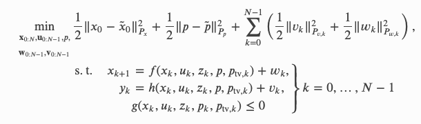image This change makes it possible for the user to decide, which measurements are enforced and which can be perturbed. A typical example would be to ensure that input “measurements” are completely trusted.

Simulator with disturbances

The newly introduced measurement noise and the existing process noise are now used within the simulator. With each call of Simulator.make_step values can be passed to obtain an imperfectly simulated and measured system..

Documentation

• Release notes are now included in the documentation. They are autogenerated from the Github release notes which can be accessed via Rest API.
• The release notes are appended with a section that includes a download link for the example files that were written for the respective versions.
• Installation instructions now refer to these download links. This solves #62 .
• Added new section Example gallery, explaining the supplied examples in do-mpc in Jupyter Notebooks (rendered on readthedocs)
• Added new section Background with various articles explaining the mathematics behind do-mpc.
• Parameter collocation_ni in MPC/MHE is now explained more clearly.

Minor changes

• Renamed model.setup_model() -> model.setup()in all examples. This adresses #38
• opt_p_num and opt_x_num for MHE/MPC are now instance properties instead of class attributes. They still appear in the documentation and can be used as before. Having them as class attributes can lead to problems when multiple classes are live during the same session.

Example files

Please download the example files for release do-mpc v4.0.0 here.

do-mpc v4.0.0-beta3

Major changes

Data

• New __getitem__ method to conveniently retrieve values from Data object (details here)
• New MPCData class (which inherits form Data). This adds the prediction method, which can be used to query the optimal trajectories. Details here.

Both methods were previously (in a slightly different form) in the Graphics module. They are still used in this class but can also be convenient under different circumstances.

Graphics

The Graphics module is now initialized with a specific Data instance (e.g. mpc.data). Each Data class has their own Graphics class (if it is supposed to be displayed). Compared to the previous implementation, we now initialize all lines that are supposed to be plotted (and store them in pred_lines and result_lines). During runtime, the data on these lines is getting updated.

• Added new structure class in do_mpc.tools. Used for tracking the new Graphics properties: pred_lines and result_lines.
• The properties pred_lines and result_lines can be used to retrieve line instances with power indices. Line instances can be easily configured (linestyle, alpha, color etc.)

Process noise

Process noise can be added to rhs of Model class: link

This is solving issue #53 .

This change was necessary to allow for the more natural MHE formulation where the process noise is penalised in the cost function. The user can define for each state (vector) individually if this is intended or not.

As a consequence of this change I had to introduce the new variable w throughout do-mpc. For the MPC and simulator module this is without effect.

The main difference is here

Remark: The change also allows to estimate parameters that change over time (e.g. environmental influences). Our regular estimated parameters are constant over the entire MHE horizon, which is not always valid. To estimate varying parameters, they should be defined as states with unknown dynamics. Concretely, their RHS is zero (for ODEs) and they have a high process noise.

Symbolic variables for MHE weighting matrices

As originally intended, it is now possible to have symbolic matrices as MHE tuning factors. The result of this change can be seen in the rotating_oscillating_masses example.

The symbolic variables are defined in the do-mpc Model where typically, you want to have P_x and P_p as parameters and P_y and P_w as time-varying parameters. Example of their definition.

and here they are used.

The purpose of using symbolic weighting is of course to update them at each iteration. Since they are parameters and time-varying parameters respectively, this is done with the set_p_fun and set_tvp_fun method of the MHE: link

Note that in the example above, we don’t actually need varying weighting matrices and the returned values are in fact constant. This can be seen as a proof of concept.

This change had some other implications. Most notably, having additional parameters interferes with the multi-stage robust MPC module. Where we previously had to pass a number of scenarios for each defined parameter. Since parameters for the MHE are irrelevant for MPC the API for the call set_uncertainty_values has changed: link

The new API is fully backwards compatible. However, it is much more intuitive now. The function is called with keyword arguments, where each keyword refers to one uncertain parameter (note that we can ignore the parameters that are irrelevant). In practice this looks something like this

Example files

Please download the example files for release do-mpc v4.0.0-beta3 here.

do-mpc v4.0.0-beta2

Error in release. Immediately replaced with beta3.

do-mpc v4.0.0-beta1

Major changes

• We are now explicitly pointing out attributes of the Model such as states, inputs, etc. These should be used to obtain these attributes and replace the previous get_variables method which is now depreciated. The Model also supports a __get_variable__ call now to conveniently select items.
• setup_model is replaced by setup to be more consistent with other setup methods. The old method is still available and shows a depreciation warning.
• The MHE now supports the set_default_objective method.

Bug fixes

• The MHE formulation had an error in the make_step method. We used the wrong time step from the previous solution to compute the arrival cost.

Other changes

• Spelling in documentation
• New guide about installing HSL linear solver
• Credits in documentation

Example files

Please download the example files for release do-mpc v4.0.0-beta1 here.

do-mpc v4.0.0-beta

do-mpc has undergone a massive overhaul and comes with a completely new interface, new features and a comprehensive documentation.

Please note that previously written code is not compatible with do-mpc 4.0.0. If you want to continue working with older code please use version 3.0.0.

This is the beta release of version 4.0.0. We expect minor modifications and bug fixes in the near future.

Please see our documentation on our new project homepage www.do-mpc.com for a full list of features.

Example files

Please download the example files for release do-mpc v4.0.0-beta here.

do-mpc v3.0.0

Main modifications

• Support for CasADi version 3.4.4
• Support for time-varying parameters
• Support for discrete-time systems

do-mpc v2.0.0

Compatible with CasADi 3.0.0

do-mpc version 1.0.0

Batch Bioreactor

In this Jupyter Notebook we illustrate the example batch_reactor.

Open an interactive online Jupyter Notebook with this content on Binder:

The example consists of the three modules template_model.py, which describes the system model, template_mpc.py, which defines the settings for the control and template_simulator.py, which sets the parameters for the simulator. The modules are used in main.py for the closed-loop execution of the controller.

In the following the different parts are presented. But first, we start by importing basic modules and do-mpc.

import numpy as np
import sys
from casadi import *

# Add do_mpc to path. This is not necessary if it was installed via pip
sys.path.append('../../../')

# Import do_mpc package:
import do_mpc

Model

In the following we will present the configuration, setup and connection between these blocks, starting with the model.

The considered model of the batch bioreactor is continuous and has 4 states and 1 control input, which are depicted below:

The model is initiated by:

model_type = 'continuous' # either 'discrete' or 'continuous'
model = do_mpc.model.Model(model_type)

States and control inputs

The four states are concentration of the biomass \(X_{\text{s}}\), the concentration of the substrate \(S_{\text{s}}\), the concentration of the product \(P_{\text{s}}\) and the volume \(V_{\text{s}}\):

# States struct (optimization variables):
X_s = model.set_variable('_x',  'X_s')
S_s = model.set_variable('_x',  'S_s')
P_s = model.set_variable('_x',  'P_s')
V_s = model.set_variable('_x',  'V_s')

The control input is the feed flow rate \(u_{\text{inp}}\) of \(S_{\text{s}}\):

# Input struct (optimization variables):
inp = model.set_variable('_u',  'inp')

ODE and parameters

The system model is described by the ordinary differential equation:

\begin{align} \dot{X}_{\text{s}} &=\mu(S_{\text{s}})X_{\text{s}}-\frac{u_{\text{inp}}}{V_{\text{s}}}X_{\text{s}},\\ \dot{S}_{\text{s}} &=-\frac{\mu(S_{\text{s}})X_{\text{s}}}{Y_{\text{x}}}-\frac{vX_{\text{s}}}{Y_{\text{p}}}+\frac{u_{\text{inp}}}{V_{\text{s}}}(S_{\text{in}}-S_{\text{s}}),\\ \dot{P}_{\text{s}} &=vX_{\text{s}}-\frac{u_{\text{inp}}}{V_{\text{s}}}P_{\text{s}},\\ \dot{V}_{\text{s}} &=u_{\text{inp}},\\ \end{align}

where:

\begin{align} \mu(S_{\text{s}})&=\frac{\mu_{\text{m}} S_{\text{s}}}{K_{\text{m}}+S_{\text{s}}+(S_{\text{s}}^2/K_{\text{i}})}, \end{align}

\(S_{\text{in}}\) is the inlet substrate concentration, \(\mu_{\text{m}}\), \(K_{\text{m}}\), \(K_{\text{i}}\) and \(v\) are kinetic parameters \(Y_{\text{x}}\) and \(Y_{\text{p}}\) are yield coefficients. The inlet substrate concentration \(S_{\text{in}}\) and the \(Y_{\text{x}}\) are uncertain while the rest of the parameters is considered certain:

# Certain parameters
mu_m  = 0.02
K_m   = 0.05
K_i   = 5.0
v_par = 0.004
Y_p   = 1.2

# Uncertain parameters:
Y_x  = model.set_variable('_p',  'Y_x')
S_in = model.set_variable('_p', 'S_in')

In the next step, the ODE for each state is set:

# Auxiliary term
mu_S = mu_m*S_s/(K_m+S_s+(S_s**2/K_i))

# Differential equations
model.set_rhs('X_s', mu_S*X_s - inp/V_s*X_s)
model.set_rhs('S_s', -mu_S*X_s/Y_x - v_par*X_s/Y_p + inp/V_s*(S_in-S_s))
model.set_rhs('P_s', v_par*X_s - inp/V_s*P_s)
model.set_rhs('V_s', inp)

Finally, the model setup is completed:

# Build the model
model.setup()

Controller

Next, the controller is configured. First, one member of the mpc class is generated with the prediction model defined above:

mpc = do_mpc.controller.MPC(model)

We choose the prediction horizon n_horizon, set the robust horizon n_robust to 3. The time step t_step is set to one second and parameters of the applied discretization scheme orthogonal collocation are as seen below:

setup_mpc = {
    'n_horizon': 20,
    'n_robust': 1,
    'open_loop': 0,
    't_step': 1.0,
    'state_discretization': 'collocation',
    'collocation_type': 'radau',
    'collocation_deg': 2,
    'collocation_ni': 2,
    'store_full_solution': True,
    # Use MA27 linear solver in ipopt for faster calculations:
    #'nlpsol_opts': {'ipopt.linear_solver': 'MA27'}
}

mpc.set_param(**setup_mpc)

Objective

The batch bioreactor is used to produce penicillin. Hence, the objective of the controller is to maximize the concentration of the product \(P_{\text{s}}\). Additionally, we add a penalty on input changes, to obtain a smooth control performance.

mterm = -model.x['P_s'] # stage cost
lterm = -model.x['P_s'] # terminal cost

mpc.set_objective(mterm=mterm, lterm=lterm)
mpc.set_rterm(inp=1.0) # penalty on input changes

Constraints

In the next step, the constraints of the control problem are set. In this case, there are only upper and lower bounds for each state and the input:

# lower bounds of the states
mpc.bounds['lower', '_x', 'X_s'] = 0.0
mpc.bounds['lower', '_x', 'S_s'] = -0.01
mpc.bounds['lower', '_x', 'P_s'] = 0.0
mpc.bounds['lower', '_x', 'V_s'] = 0.0

# upper bounds of the states
mpc.bounds['upper', '_x','X_s'] = 3.7
mpc.bounds['upper', '_x','P_s'] = 3.0

# upper and lower bounds of the control input
mpc.bounds['lower','_u','inp'] = 0.0
mpc.bounds['upper','_u','inp'] = 0.2

Uncertain values

The explicit values of the two uncertain parameters \(Y_{\text{x}}\) and \(S_{\text{in}}\), which are considered in the scenario tree, are given by:

Y_x_values = np.array([0.5, 0.4, 0.3])
S_in_values = np.array([200.0, 220.0, 180.0])

mpc.set_uncertainty_values([Y_x_values, S_in_values])

This means with n_robust=1, that 9 different scenarios are considered. The setup of the MPC controller is concluded by:

mpc.setup()

Estimator

We assume, that all states can be directly measured (state-feedback):

estimator = do_mpc.estimator.StateFeedback(model)

Simulator

To create a simulator in order to run the MPC in a closed-loop, we create an instance of the do-mpc simulator which is based on the same model:

simulator = do_mpc.simulator.Simulator(model)

For the simulation, we use the time step t_step as for the optimizer:

params_simulator = {
    'integration_tool': 'cvodes',
    'abstol': 1e-10,
    'reltol': 1e-10,
    't_step': 1.0
}

simulator.set_param(**params_simulator)

Realizations of uncertain parameters

For the simulatiom, it is necessary to define the numerical realizations of the uncertain parameters in p_num. First, we get the structure of the uncertain parameters:

p_num = simulator.get_p_template()

We define a function which is called in each simulation step, which gives the current realization of the uncertain parameters, with respect to defined inputs (in this case t_now):

p_num['Y_x'] = 0.4
p_num['S_in'] = 200.0

# function definition
def p_fun(t_now):
    return p_num

# Set the user-defined function above as the function for the realization of the uncertain parameters
simulator.set_p_fun(p_fun)

By defining p_fun as above, the function will always return the same values. To finish the configuration of the simulator, call:

simulator.setup()

Closed-loop simulation

For the simulation of the MPC configured for the batch bioreactor, we inspect the file main.py. We define the initial state of the system and set for all parts of the closed-loop configuration:

# Initial state
X_s_0 = 1.0 # Concentration biomass [mol/l]
S_s_0 = 0.5 # Concentration substrate [mol/l]
P_s_0 = 0.0 # Concentration product [mol/l]
V_s_0 = 120.0 # Volume inside tank [m^3]
x0 = np.array([X_s_0, S_s_0, P_s_0, V_s_0])

# Set for controller, simulator and estimator
mpc.x0 = x0
simulator.x0 = x0
estimator.x0 = x0
mpc.set_initial_guess()

Prepare visualization

For the visualization of the control performance, we first import matplotlib and change some basic settings:

import matplotlib.pyplot as plt
plt.ion()
from matplotlib import rcParams
rcParams['text.usetex'] = True
rcParams['text.latex.preamble'] = [r'\usepackage{amsmath}',r'\usepackage{siunitx}']
rcParams['axes.grid'] = True
rcParams['lines.linewidth'] = 2.0
rcParams['axes.labelsize'] = 'xx-large'
rcParams['xtick.labelsize'] = 'xx-large'
rcParams['ytick.labelsize'] = 'xx-large'

We use the plotting capabilities, which are included in do-mpc. The mpc_graphics contain information like the current estimated state and the predicted trajectory of the states and inputs based on the solution of the control problem. The sim_graphics contain the information about the simulated evaluation of the system.

mpc_graphics = do_mpc.graphics.Graphics(mpc.data)
sim_graphics = do_mpc.graphics.Graphics(simulator.data)

A figure containing the 4 states and the control input are created:

%%capture
fig, ax = plt.subplots(5, sharex=True, figsize=(16,9))
fig.align_ylabels()

for g in [sim_graphics,mpc_graphics]:
    # Plot the state on axis 1 to 4:
    g.add_line(var_type='_x', var_name='X_s', axis=ax[0], color='#1f77b4')
    g.add_line(var_type='_x', var_name='S_s', axis=ax[1], color='#1f77b4')
    g.add_line(var_type='_x', var_name='P_s', axis=ax[2], color='#1f77b4')
    g.add_line(var_type='_x', var_name='V_s', axis=ax[3], color='#1f77b4')

    # Plot the control input on axis 5:
    g.add_line(var_type='_u', var_name='inp', axis=ax[4], color='#1f77b4')


ax[0].set_ylabel(r'$X_s~[\si[per-mode=fraction]{\mole\per\litre}]$')
ax[1].set_ylabel(r'$S_s~[\si[per-mode=fraction]{\mole\per\litre}]$')
ax[2].set_ylabel(r'$P_s~[\si[per-mode=fraction]{\mole\per\litre}]$')
ax[3].set_ylabel(r'$V_s~[\si[per-mode=fraction]{\mole\per\litre}]$')
ax[4].set_ylabel(r'$u_{\text{inp}}~[\si[per-mode=fraction]{\cubic\metre\per\minute}]$')
ax[4].set_xlabel(r'$t~[\si[per-mode=fraction]{\minute}]$')

Run closed-loop

The closed-loop system is now simulated for 50 steps (and the ouput of the optimizer is suppressed):

%%capture
n_steps = 100
for k in range(n_steps):
    u0 = mpc.make_step(x0)
    y_next = simulator.make_step(u0)
    x0 = estimator.make_step(y_next)

Results

The next cell converts the results of the closed-loop MPC simulation into a gif (might take a few minutes):

from matplotlib.animation import FuncAnimation, FFMpegWriter, ImageMagickWriter

# The function describing the gif:
def update(t_ind):
    sim_graphics.plot_results(t_ind)
    mpc_graphics.plot_predictions(t_ind)
    mpc_graphics.reset_axes()


anim = FuncAnimation(fig, update, frames=n_steps, repeat=False)
gif_writer = ImageMagickWriter(fps=10)
anim.save('anim_batch_reactor_final.gif', writer=gif_writer)

The result is shown below, where solid lines are the recorded trajectories and dashed lines are the predictions of the scenarios:

Continuous stirred tank reactor (CSTR)

In this Jupyter Notebook we illustrate the example CSTR.

Open an interactive online Jupyter Notebook with this content on Binder:

The example consists of the three modules template_model.py, which describes the system model, template_mpc.py, which defines the settings for the control and template_simulator.py, which sets the parameters for the simulator. The modules are used in main.py for the closed-loop execution of the controller. The file post_processing.py is used for the visualization of the closed-loop control run. One exemplary result will be presented at the end of this tutorial as a gif.

In the following the different parts are presented. But first, we start by importing basic modules and do-mpc.

import numpy as np
import sys
from casadi import *

# Add do_mpc to path. This is not necessary if it was installed via pip
sys.path.append('../../../')

# Import do_mpc package:
import do_mpc

import matplotlib.pyplot as plt

Model

In the following we will present the configuration, setup and connection between these blocks, starting with the model. The considered model of the CSTR is continuous and has 4 states and 2 control inputs. The model is initiated by:

model_type = 'continuous' # either 'discrete' or 'continuous'
model = do_mpc.model.Model(model_type)

States and control inputs

The four states are concentration of reactant A (\(C_{\text{A}}\)), the concentration of reactant B (\(C_{\text{B}}\)), the temperature inside the reactor (\(T_{\text{R}}\)) and the temperature of the cooling jacket (\(T_{\text{K}}\)):

# States struct (optimization variables):
C_a = model.set_variable(var_type='_x', var_name='C_a', shape=(1,1))
C_b = model.set_variable(var_type='_x', var_name='C_b', shape=(1,1))
T_R = model.set_variable(var_type='_x', var_name='T_R', shape=(1,1))
T_K = model.set_variable(var_type='_x', var_name='T_K', shape=(1,1))

The control inputs are the feed \(F\) and the heat flow \(\dot{Q}\):

# Input struct (optimization variables):
F = model.set_variable(var_type='_u', var_name='F')
Q_dot = model.set_variable(var_type='_u', var_name='Q_dot')

ODE and parameters

The system model is described by the ordinary differential equation:

\begin{align} \dot{C}_{\text{A}} &= F \cdot (C_{\text{A},0} - C_{\text{A}}) - k_1 \cdot C_{\text{A}} - k_3 \cdot C_{\text{A}}^2, \\ \dot{C}_{\text{B}} &= F \cdot C_{\text{B}} + k_1 \cdot C_{\text{A}} - k_2 \cdot C_{\text{B}}, \\ \dot{T}_{\text{R}} &= \frac{k_1 \cdot C_{\text{A}} \cdot H_{\text{R},ab} + k_2 \cdot C_{\text{B}} \cdot H_{\text{R},bc} + k_3 \cdot C_{\text{A}}^2 \cdot H_{\text{R},ad}} {-\rho \cdot c_p}\\ &+ F \cdot (T_{\text{in}} - T_{\text{R}}) + \frac{K_w \cdot A_{\text{R}} \cdot(T_{\text{K}}-T_{\text{R}})}{\rho \cdot c_p \cdot V_{\text{R}}}, \\ \dot{T}_{\text{K}} &= \frac{\dot{Q} + k_w \cdot A_{\text{R}} \cdot T_{\text{dif}}}{m_k \cdot C_{p,k}}, \end{align}

where

\begin{align} k_1 &= \beta \cdot k_{0,\text{ab}} \cdot \exp\left(\frac{-E_{\text{A},\text{ab}}}{T_{\text{R}}+273.15}\right), \\ k_1 &= k_{0,\text{bc}} \cdot \exp \left( \frac{-E_{\text{A},\text{bc}}}{T_{\text{R}}+273.15} \right), \\ k_3 &= k_{0,\text{ad}} \cdot \exp \left( \frac{-\alpha \cdot E_{\text{A},\text{ad}}}{T_{\text{R}}+273.15} \right). \end{align}

The parameters \(\alpha\) and \(\beta\) are uncertain while the rest of the parameters is considered certain:

# Certain parameters
K0_ab = 1.287e12 # K0 [h^-1]
K0_bc = 1.287e12 # K0 [h^-1]
K0_ad = 9.043e9 # K0 [l/mol.h]
R_gas = 8.3144621e-3 # Universal gas constant
E_A_ab = 9758.3*1.00 #* R_gas# [kj/mol]
E_A_bc = 9758.3*1.00 #* R_gas# [kj/mol]
E_A_ad = 8560.0*1.0 #* R_gas# [kj/mol]
H_R_ab = 4.2 # [kj/mol A]
H_R_bc = -11.0 # [kj/mol B] Exothermic
H_R_ad = -41.85 # [kj/mol A] Exothermic
Rou = 0.9342 # Density [kg/l]
Cp = 3.01 # Specific Heat capacity [kj/Kg.K]
Cp_k = 2.0 # Coolant heat capacity [kj/kg.k]
A_R = 0.215 # Area of reactor wall [m^2]
V_R = 10.01 #0.01 # Volume of reactor [l]
m_k = 5.0 # Coolant mass[kg]
T_in = 130.0 # Temp of inflow [Celsius]
K_w = 4032.0 # [kj/h.m^2.K]
C_A0 = (5.7+4.5)/2.0*1.0 # Concentration of A in input Upper bound 5.7 lower bound 4.5 [mol/l]

# Uncertain parameters:
alpha = model.set_variable(var_type='_p', var_name='alpha')
beta = model.set_variable(var_type='_p', var_name='beta')

In the next step, we formulate the \(k_i\)-s:

# Auxiliary terms
K_1 = beta * K0_ab * exp((-E_A_ab)/((T_R+273.15)))
K_2 =  K0_bc * exp((-E_A_bc)/((T_R+273.15)))
K_3 = K0_ad * exp((-alpha*E_A_ad)/((T_R+273.15)))

Additionally, we define an artificial variable of interest, that is not a state of the system, but will be later used for plotting:

T_dif = model.set_expression(expr_name='T_dif', expr=T_R-T_K)

WIth the help ot the \(k_i\)-s and \(T_{\text{dif}}\) we can define the ODEs:

model.set_rhs('C_a', F*(C_A0 - C_a) -K_1*C_a - K_3*(C_a**2))
model.set_rhs('C_b', -F*C_b + K_1*C_a - K_2*C_b)
model.set_rhs('T_R', ((K_1*C_a*H_R_ab + K_2*C_b*H_R_bc + K_3*(C_a**2)*H_R_ad)/(-Rou*Cp)) + F*(T_in-T_R) +(((K_w*A_R)*(-T_dif))/(Rou*Cp*V_R)))
model.set_rhs('T_K', (Q_dot + K_w*A_R*(T_dif))/(m_k*Cp_k))

Finally, the model setup is completed:

# Build the model
model.setup()

Controller

Next, the model predictive controller is configured. First, one member of the mpc class is generated with the prediction model defined above:

mpc = do_mpc.controller.MPC(model)

We choose the prediction horizon n_horizon, set the robust horizon n_robust to 1. The time step t_step is set to one second and parameters of the applied discretization scheme orthogonal collocation are as seen below:

setup_mpc = {
    'n_horizon': 20,
    'n_robust': 1,
    'open_loop': 0,
    't_step': 0.005,
    'state_discretization': 'collocation',
    'collocation_type': 'radau',
    'collocation_deg': 2,
    'collocation_ni': 2,
    'store_full_solution': True,
    # Use MA27 linear solver in ipopt for faster calculations:
    #'nlpsol_opts': {'ipopt.linear_solver': 'MA27'}
}

mpc.set_param(**setup_mpc)

Because the magnitude of the states and inputs is very different, we introduce scaling factors:

mpc.scaling['_x', 'T_R'] = 100
mpc.scaling['_x', 'T_K'] = 100
mpc.scaling['_u', 'Q_dot'] = 2000
mpc.scaling['_u', 'F'] = 100

Objective

The goal of the CSTR is to obtain a mixture with a concentration of \(C_{\text{B,ref}} = 0.6\) mol/l. Additionally, we add a penalty on input changes for both control inputs, to obtain a smooth control performance.

_x = model.x
mterm = (_x['C_b'] - 0.6)**2 # terminal cost
lterm = (_x['C_b'] - 0.6)**2 # stage cost

mpc.set_objective(mterm=mterm, lterm=lterm)

mpc.set_rterm(F=0.1, Q_dot = 1e-3) # input penalty

Constraints

In the next step, the constraints of the control problem are set. In this case, there are only upper and lower bounds for each state and the input:

# lower bounds of the states
mpc.bounds['lower', '_x', 'C_a'] = 0.1
mpc.bounds['lower', '_x', 'C_b'] = 0.1
mpc.bounds['lower', '_x', 'T_R'] = 50
mpc.bounds['lower', '_x', 'T_K'] = 50

# upper bounds of the states
mpc.bounds['upper', '_x', 'C_a'] = 2
mpc.bounds['upper', '_x', 'C_b'] = 2
mpc.bounds['upper', '_x', 'T_K'] = 140

# lower bounds of the inputs
mpc.bounds['lower', '_u', 'F'] = 5
mpc.bounds['lower', '_u', 'Q_dot'] = -8500

# upper bounds of the inputs
mpc.bounds['upper', '_u', 'F'] = 100
mpc.bounds['upper', '_u', 'Q_dot'] = 0.0

If a constraint is not critical, it is possible to implement it as a soft constraint. This means, that a small violation of the constraint does not render the optimization infeasible. Instead, a penalty term is added to the objective. Soft constraints can always be applied, if small violations can be accepted and it might even be necessary to apply MPC in a safe way (by avoiding avoiding numerical instabilities). In this case, we define the upper bounds of the reactor temperature as a soft constraint by using mpc.set_nl_cons().

mpc.set_nl_cons('T_R', _x['T_R'], ub=140, soft_constraint=True, penalty_term_cons=1e2)

SX((T_R-eps_T_R))

Uncertain values

The explicit values of the two uncertain parameters \(\alpha\) and \(\beta\), which are considered in the scenario tree, are given by:

alpha_var = np.array([1., 1.05, 0.95])
beta_var = np.array([1., 1.1, 0.9])

mpc.set_uncertainty_values([alpha_var, beta_var])

This means with n_robust=1, that 9 different scenarios are considered. The setup of the MPC controller is concluded by:

mpc.setup()

Estimator

We assume, that all states can be directly measured (state-feedback):

estimator = do_mpc.estimator.StateFeedback(model)

Simulator

To create a simulator in order to run the MPC in a closed-loop, we create an instance of the do-mpc simulator which is based on the same model:

simulator = do_mpc.simulator.Simulator(model)

For the simulation, we use the same time step t_step as for the optimizer:

params_simulator = {
    'integration_tool': 'cvodes',
    'abstol': 1e-10,
    'reltol': 1e-10,
    't_step': 0.005
}

simulator.set_param(**params_simulator)

Realizations of uncertain parameters

For the simulatiom, it is necessary to define the numerical realizations of the uncertain parameters in p_num and the time-varying parameters in tvp_num. First, we get the structure of the uncertain and time-varying parameters:

p_num = simulator.get_p_template()
tvp_num = simulator.get_tvp_template()

We define two functions which are called in each simulation step, which return the current realizations of the parameters, with respect to defined inputs (in this case t_now):

# function for time-varying parameters
def tvp_fun(t_now):
    return tvp_num

# uncertain parameters
p_num['alpha'] = 1
p_num['beta'] = 1
def p_fun(t_now):
    return p_num

These two custum functions are used in the simulation via:

simulator.set_tvp_fun(tvp_fun)
simulator.set_p_fun(p_fun)

By defining p_fun as above, the function will always return the value 1.0 for both \(\alpha\) and \(\beta\). To finish the configuration of the simulator, call:

simulator.setup()

Closed-loop simulation

For the simulation of the MPC configured for the CSTR, we inspect the file main.py. We define the initial state of the system and set it for all parts of the closed-loop configuration:

# Set the initial state of mpc, simulator and estimator:
C_a_0 = 0.8 # This is the initial concentration inside the tank [mol/l]
C_b_0 = 0.5 # This is the controlled variable [mol/l]
T_R_0 = 134.14 #[C]
T_K_0 = 130.0 #[C]
x0 = np.array([C_a_0, C_b_0, T_R_0, T_K_0]).reshape(-1,1)

mpc.x0 = x0
simulator.x0 = x0
estimator.x0 = x0

mpc.set_initial_guess()

Now, we simulate the closed-loop for 50 steps (and suppress the output of the cell with the magic command %%capture):

%%capture
for k in range(50):
    u0 = mpc.make_step(x0)
    y_next = simulator.make_step(u0)
    x0 = estimator.make_step(y_next)

Animating the results

To animate the results, we first configure the do-mpc graphics object, which is initiated with the respective data object:

mpc_graphics = do_mpc.graphics.Graphics(mpc.data)

We quickly configure Matplotlib.

from matplotlib import rcParams
rcParams['axes.grid'] = True
rcParams['font.size'] = 18

We then create a figure, configure which lines to plot on which axis and add labels.

%%capture
fig, ax = plt.subplots(5, sharex=True, figsize=(16,12))
# Configure plot:
mpc_graphics.add_line(var_type='_x', var_name='C_a', axis=ax[0])
mpc_graphics.add_line(var_type='_x', var_name='C_b', axis=ax[0])
mpc_graphics.add_line(var_type='_x', var_name='T_R', axis=ax[1])
mpc_graphics.add_line(var_type='_x', var_name='T_K', axis=ax[1])
mpc_graphics.add_line(var_type='_aux', var_name='T_dif', axis=ax[2])
mpc_graphics.add_line(var_type='_u', var_name='Q_dot', axis=ax[3])
mpc_graphics.add_line(var_type='_u', var_name='F', axis=ax[4])
ax[0].set_ylabel('c [mol/l]')
ax[1].set_ylabel('T [K]')
ax[2].set_ylabel('$\Delta$ T [K]')
ax[3].set_ylabel('Q [kW]')
ax[4].set_ylabel('Flow [l/h]')
ax[4].set_xlabel('time [h]')

Some “cosmetic” modifications are easily achieved with the structure pred_lines and result_lines.

# Update properties for all prediction lines:
for line_i in mpc_graphics.pred_lines.full:
    line_i.set_linewidth(2)
# Highlight nominal case:
for line_i in np.sum(mpc_graphics.pred_lines['_x', :, :,0]):
    line_i.set_linewidth(5)
for line_i in np.sum(mpc_graphics.pred_lines['_u', :, :,0]):
    line_i.set_linewidth(5)
for line_i in np.sum(mpc_graphics.pred_lines['_aux', :, :,0]):
    line_i.set_linewidth(5)

# Add labels
label_lines = mpc_graphics.result_lines['_x', 'C_a']+mpc_graphics.result_lines['_x', 'C_b']
ax[0].legend(label_lines, ['C_a', 'C_b'])
label_lines = mpc_graphics.result_lines['_x', 'T_R']+mpc_graphics.result_lines['_x', 'T_K']
ax[1].legend(label_lines, ['T_R', 'T_K'])

fig.align_ylabels()

After importing the necessary package:

from matplotlib.animation import FuncAnimation, ImageMagickWriter

We obtain the animation with:

def update(t_ind):
    print('Writing frame: {}.'.format(t_ind), end='\r')
    mpc_graphics.plot_results(t_ind=t_ind)
    mpc_graphics.plot_predictions(t_ind=t_ind)
    mpc_graphics.reset_axes()
    lines = mpc_graphics.result_lines.full
    return lines

n_steps = mpc.data['_time'].shape[0]


anim = FuncAnimation(fig, update, frames=n_steps, blit=True)

gif_writer = ImageMagickWriter(fps=5)
anim.save('anim_CSTR.gif', writer=gif_writer)

Writing frame: 49.

Recorded trajectories are shown as solid lines, whereas predictions are dashed. We highlight the nominal prediction with a thicker line.

Industrial polymerization reactor

In this Jupyter Notebook we illustrate the example industrial_poly.

Open an interactive online Jupyter Notebook with this content on Binder:

The example consists of the three modules template_model.py, which describes the system model, template_mpc.py, which defines the settings for the control and template_simulator.py, which sets the parameters for the simulator. The modules are used in main.py for the closed-loop execution of the controller.

In the following the different parts are presented. But first, we start by importing basic modules and do-mpc.

import numpy as np
import matplotlib.pyplot as plt
import sys
from casadi import *

# Add do_mpc to path. This is not necessary if it was installed via pip
sys.path.append('../../../')

# Import do_mpc package:
import do_mpc

Model

In the following we will present the configuration, setup and connection between these blocks, starting with the model. The considered model of the industrial reactor is continuous and has 10 states and 3 control inputs. The model is initiated by:

model_type = 'continuous' # either 'discrete' or 'continuous'
model = do_mpc.model.Model(model_type)

System description

The system consists of a reactor into which nonomer is fed. The monomerturns into a polymer via a very exothermic chemical reaction. The reactor is equipped with a jacket and with an External Heat Exchanger(EHE) that can both be used to control the temperature inside the reactor. A schematic representation of the system is presented below:

The process is modeled by a set of 8 ordinary differential equations (ODEs):

\begin{align} \dot{m}_{\text{W}} &= \ \dot{m}_{\text{F}}\, \omega_{\text{W,F}} \\ \dot{m}_{\text{A}} &= \ \dot{m}_{\text{F}} \omega_{\text{A,F}}-k_{\text{R1}}\, m_{\text{A,R}}-k_{\text{R2}}\, m_{\text{AWT}}\, m_{\text{A}}/m_{\text{ges}} , \\ \dot{m}_{\text{P}} &= \ k_{\text{R1}} \, m_{\text{A,R}}+p_{1}\, k_{\text{R2}}\, m_{\text{AWT}}\, m_{\text{A}}/ m_{\text{ges}}, \\ \dot{T}_{\text{R}} &= \ 1/(c_{\text{p,R}} m_{\text{ges}})\; [\dot{m}_{\text{F}} \; c_{\text{p,F}}\left(T_{\text{F}}-T_{\text{R}}\right) +\Delta H_{\text{R}} k_{\text{R1}} m_{\text{A,R}}-k_{\text{K}} A\left(T_{\text{R}}-T_{\text{S}}\right) \\ &- \dot{m}_{\text{AWT}} \,c_{\text{p,R}}\left(T_{\text{R}}-T_{\text{EK}}\right)],\notag\\ \dot{T}_{S} &= 1/(c_{\text{p,S}} m_{\text{S}}) \;[k_{\text{K}} A\left(T_{\text{R}}-T_{\text{S}}\right)-k_{\text{K}} A\left(T_{\text{S}}-T_{\text{M}}\right)], \notag\\ \dot{T}_{\text{M}} &= 1/(c_{\text{p,W}} m_{\text{M,KW}})\;[\dot{m}_{\text{M,KW}}\, c_{\text{p,W}}\left(T_{\text{M}}^{\text{IN}}-T_{\text{M}}\right) \\ &+ k_{\text{K}} A\left(T_{\text{S}}-T_{\text{M}}\right)]+k_{\text{K}} A\left(T_{\text{S}}-T_{\text{M}}\right)], \\ \dot{T}_{\text{EK}}&= 1/(c_{\text{p,R}} m_{\text{AWT}})\;[\dot{m}_{\text{AWT}} c_{\text{p,W}}\left(T_{\text{R}}-T_{\text{EK}}\right)-\alpha\left(T_{\text{EK}}-T_{\text{AWT}}\right) \\ &+ k_{\text{R2}}\, m_{\text{A}}\, m_{\text{AWT}}\Delta H_{\text{R}}/m_{\text{ges}}], \notag\\ \dot{T}_{\text{AWT}} &= [\dot{m}_{\text{AWT,KW}} \,c_{\text{p,W}}\,(T_{\text{AWT}}^{\text{IN}}-T_{\text{AWT}})-\alpha\left(T_{\text{AWT}}-T_{\text{EK}}\right)]/(c_{\text{p,W}} m_{\text{AWT,KW}}), \end{align}

where

\begin{align} U &= m_{\text{P}}/(m_{\text{A}}+m_{\text{P}}), \\ m_{\text{ges}} &= \ m_{\text{W}}+m_{\text{A}}+m_{\text{P}}, \\ k_{\text{R1}} &= \ k_{0} e^{\frac{-E_{a}}{R (T_{\text{R}}+273.15)}}\left(k_{\text{U1}}\left(1-U\right)+k_{\text{U2}} U\right), \\ k_{\text{R2}} &= \ k_{0} e^{\frac{-E_{a}}{R (T_{\text{EK}}+273.15)}}\left(k_{\text{U1}}\left(1-U\right)+k_{\text{U2}} U\right), \\ k_{\text{K}} &= (m_{\text{W}}k_{\text{WS}}+m_{\text{A}}k_{\text{AS}}+m_{\text{P}}k_{\text{PS}})/m_{\text{ges}},\\ m_{\text{A,R}} &= m_\text{A}-m_\text{A} m_{\text{AWT}}/m_{\text{ges}}. \end{align}

The model includes mass balances for the water, monomer and product hold-ups (\(m_\text{W}\), \(m_\text{A}\), \(m_\text{P}\)) and energy balances for the reactor (\(T_\text{R}\)), the vessel (\(T_\text{S}\)), the jacket (\(T_\text{M}\)), the mixture in the external heat exchanger (\(T_{\text{EK}}\)) and the coolant leaving the external heat exchanger (\(T_{\text{AWT}}\)). The variable \(U\) denotes the polymer-monomer ratio in the reactor, \(m_{\text{ges}}\) represents the total mass, \(k_{\text{R1}}\) is the reaction rate inside the reactor and \(k_{\text{R2}}\) is the reaction rate in the external heat exchanger. The total heat transfer coefficient of the mixture inside the reactor is denoted as \(k_{\text{K}}\) and \(m_{\text{A,R}}\) represents the current amount of monomer inside the reactor.

The available control inputs are the feed flow \(\dot{m}_{\text{F}}\), the coolant temperature at the inlet of the jacket \(T^{\text{IN}}_{\text{M}}\) and the coolant temperature at the inlet of the external heat exchanger \(T^{\text{IN}}_{\text{AWT}}\).

An overview of the parameters are listed below:

Implementation

First, we set the certain parameters:

# Certain parameters
R           = 8.314                 #gas constant
T_F         = 25 + 273.15   #feed temperature
E_a         = 8500.0                #activation energy
delH_R      = 950.0*1.00    #sp reaction enthalpy
A_tank      = 65.0                  #area heat exchanger surface jacket 65

k_0         = 7.0*1.00              #sp reaction rate
k_U2        = 32.0                  #reaction parameter 1
k_U1        = 4.0                   #reaction parameter 2
w_WF        = .333                  #mass fraction water in feed
w_AF        = .667                  #mass fraction of A in feed

m_M_KW      = 5000.0                #mass of coolant in jacket
fm_M_KW     = 300000.0              #coolant flow in jacket 300000;
m_AWT_KW    = 1000.0                #mass of coolant in EHE
fm_AWT_KW   = 100000.0              #coolant flow in EHE
m_AWT       = 200.0                 #mass of product in EHE
fm_AWT      = 20000.0               #product flow in EHE
m_S         = 39000.0               #mass of reactor steel

c_pW        = 4.2                   #sp heat cap coolant
c_pS        = .47                   #sp heat cap steel
c_pF        = 3.0                   #sp heat cap feed
c_pR        = 5.0                   #sp heat cap reactor contents

k_WS        = 17280.0               #heat transfer coeff water-steel
k_AS        = 3600.0                #heat transfer coeff monomer-steel
k_PS        = 360.0                 #heat transfer coeff product-steel

alfa        = 5*20e4*3.6

p_1         = 1.0

and afterwards the uncertain parameters:

# Uncertain parameters:
delH_R = model.set_variable('_p', 'delH_R')
k_0 =    model.set_variable('_p', 'k_0')

The 10 states of the control problem stem from the 8 ODEs, accum_monom models the amount that has been fed to the reactor via \(\dot{m}_\text{F}^{\text{acc}} = \dot{m}_{\text{F}}\) and T_adiab (\(T_{\text{adiab}}=\frac{\Delta H_{\text{R}}}{c_{\text{p,R}}} \frac{m_{\text{A}}}{m_{\text{ges}}} + T_{\text{R}}\), hence \(\dot{T}_{\text{adiab}}=\frac{\Delta H_{\text{R}}}{m_{\text{ges}} c_{\text{p,R}}}\dot{m}_{\text{A}}- \left(\dot{m}_{\text{W}}+\dot{m}_{\text{A}}+\dot{m}_{\text{P}}\right)\left(\frac{m_{\text{A}} \Delta H_{\text{R}}}{m_{\text{ges}}^2c_{\text{p,R}}}\right)+\dot{T}_{\text{R}}\)) is a virtual variable that is important for safety aspects, as we will explain later. All states are created in do-mpc via:

# States struct (optimization variables):
m_W =         model.set_variable('_x', 'm_W')
m_A =         model.set_variable('_x', 'm_A')
m_P =         model.set_variable('_x', 'm_P')
T_R =         model.set_variable('_x', 'T_R')
T_S =         model.set_variable('_x', 'T_S')
Tout_M =      model.set_variable('_x', 'Tout_M')
T_EK =        model.set_variable('_x', 'T_EK')
Tout_AWT =    model.set_variable('_x', 'Tout_AWT')
accum_monom = model.set_variable('_x', 'accum_monom')
T_adiab =     model.set_variable('_x', 'T_adiab')

and the control inputs via:

# Input struct (optimization variables):
m_dot_f = model.set_variable('_u', 'm_dot_f')
T_in_M =  model.set_variable('_u', 'T_in_M')
T_in_EK = model.set_variable('_u', 'T_in_EK')

Before defining the ODE for each state variable, we create auxiliary terms:

# algebraic equations
U_m    = m_P / (m_A + m_P)
m_ges  = m_W + m_A + m_P
k_R1   = k_0 * exp(- E_a/(R*T_R)) * ((k_U1 * (1 - U_m)) + (k_U2 * U_m))
k_R2   = k_0 * exp(- E_a/(R*T_EK))* ((k_U1 * (1 - U_m)) + (k_U2 * U_m))
k_K    = ((m_W / m_ges) * k_WS) + ((m_A/m_ges) * k_AS) + ((m_P/m_ges) * k_PS)

The auxiliary terms are used for the more readable definition of the ODEs:

# Differential equations
dot_m_W = m_dot_f * w_WF
model.set_rhs('m_W', dot_m_W)
dot_m_A = (m_dot_f * w_AF) - (k_R1 * (m_A-((m_A*m_AWT)/(m_W+m_A+m_P)))) - (p_1 * k_R2 * (m_A/m_ges) * m_AWT)
model.set_rhs('m_A', dot_m_A)
dot_m_P = (k_R1 * (m_A-((m_A*m_AWT)/(m_W+m_A+m_P)))) + (p_1 * k_R2 * (m_A/m_ges) * m_AWT)
model.set_rhs('m_P', dot_m_P)

dot_T_R = 1./(c_pR * m_ges)   * ((m_dot_f * c_pF * (T_F - T_R)) - (k_K *A_tank* (T_R - T_S)) - (fm_AWT * c_pR * (T_R - T_EK)) + (delH_R * k_R1 * (m_A-((m_A*m_AWT)/(m_W+m_A+m_P)))))
model.set_rhs('T_R', dot_T_R)
model.set_rhs('T_S', 1./(c_pS * m_S)     * ((k_K *A_tank* (T_R - T_S)) - (k_K *A_tank* (T_S - Tout_M))))
model.set_rhs('Tout_M', 1./(c_pW * m_M_KW)  * ((fm_M_KW * c_pW * (T_in_M - Tout_M)) + (k_K *A_tank* (T_S - Tout_M))))
model.set_rhs('T_EK', 1./(c_pR * m_AWT)   * ((fm_AWT * c_pR * (T_R - T_EK)) - (alfa * (T_EK - Tout_AWT)) + (p_1 * k_R2 * (m_A/m_ges) * m_AWT * delH_R)))
model.set_rhs('Tout_AWT', 1./(c_pW * m_AWT_KW)* ((fm_AWT_KW * c_pW * (T_in_EK - Tout_AWT)) - (alfa * (Tout_AWT - T_EK))))
model.set_rhs('accum_monom', m_dot_f)
model.set_rhs('T_adiab', delH_R/(m_ges*c_pR)*dot_m_A-(dot_m_A+dot_m_W+dot_m_P)*(m_A*delH_R/(m_ges*m_ges*c_pR))+dot_T_R)

Finally, the model setup is completed:

# Build the model
model.setup()

Controller

Next, the model predictive controller is configured (in template_mpc.py). First, one member of the mpc class is generated with the prediction model defined above:

mpc = do_mpc.controller.MPC(model)

Real processes are also subject to important safety constraints that are incorporated to account for possible failures of the equipment. In this case, the maximum temperature that the reactor would reach in the case of a cooling failure is constrained to be below \(109 ^\circ\)C. The temperature that the reactor would achieve in the case of a complete cooling failure is \(T_{\text{adiab}}\), hence it needs to stay beneath \(109 ^\circ\)C.

We choose the prediction horizon n_horizon, set the robust horizon n_robust to 1. The time step t_step is set to one second and parameters of the applied discretization scheme orthogonal collocation are as seen below:

setup_mpc = {
    'n_horizon': 20,
    'n_robust': 1,
    'open_loop': 0,
    't_step': 50.0/3600.0,
    'state_discretization': 'collocation',
    'collocation_type': 'radau',
    'collocation_deg': 2,
    'collocation_ni': 2,
    'store_full_solution': True,
    # Use MA27 linear solver in ipopt for faster calculations:
    #'nlpsol_opts': {'ipopt.linear_solver': 'MA27'}
}

mpc.set_param(**setup_mpc)

Objective

The goal of the economic NMPC controller is to produce \(20680~\text{kg}\) of \(m_{\text{P}}\) as fast as possible. Additionally, we add a penalty on input changes for all three control inputs, to obtain a smooth control performance.

_x = model.x
mterm = - _x['m_P'] # terminal cost
lterm = - _x['m_P'] # stage cost

mpc.set_objective(mterm=mterm, lterm=lterm)

mpc.set_rterm(m_dot_f=0.002, T_in_M=0.004, T_in_EK=0.002) # penalty on control input changes

Constraints

The temperature at which the polymerization reaction takes place strongly influences the properties of the resulting polymer. For this reason, the temperature of the reactor should be maintained in a range of \(\pm 2.0 ^\circ\)C around the desired reaction temperature \(T_{\text{set}}=90 ^\circ\)C in order to ensure that the produced polymer has the required properties.

The initial conditions and the bounds for all states are summarized in:

and set via:

# auxiliary term
temp_range = 2.0

# lower bound states
mpc.bounds['lower','_x','m_W'] = 0.0
mpc.bounds['lower','_x','m_A'] = 0.0
mpc.bounds['lower','_x','m_P'] = 26.0

mpc.bounds['lower','_x','T_R'] = 363.15 - temp_range
mpc.bounds['lower','_x','T_S'] = 298.0
mpc.bounds['lower','_x','Tout_M'] = 298.0
mpc.bounds['lower','_x','T_EK'] = 288.0
mpc.bounds['lower','_x','Tout_AWT'] = 288.0
mpc.bounds['lower','_x','accum_monom'] = 0.0

# upper bound states
mpc.bounds['upper','_x','T_R'] = 363.15 + temp_range + 10.0
mpc.bounds['upper','_x','T_S'] = 400.0
mpc.bounds['upper','_x','Tout_M'] = 400.0
mpc.bounds['upper','_x','T_EK'] = 400.0
mpc.bounds['upper','_x','Tout_AWT'] = 400.0
mpc.bounds['upper','_x','accum_monom'] = 30000.0
mpc.bounds['upper','_x','T_adiab'] = 382.15 + 10.0

The bounds of the inputsare summarized below:

and set via:

# lower bound inputs
mpc.bounds['lower','_u','m_dot_f'] = 0.0
mpc.bounds['lower','_u','T_in_M'] = 333.15
mpc.bounds['lower','_u','T_in_EK'] = 333.15

# upper bound inputs
mpc.bounds['upper','_u','m_dot_f'] = 3.0e4
mpc.bounds['upper','_u','T_in_M'] = 373.15
mpc.bounds['upper','_u','T_in_EK'] = 373.15

Scaling

Because the magnitudes of the states and inputs are very different, the performance of the optimizer can be enhanced by properly scaling the states and inputs:

# states
mpc.scaling['_x','m_W'] = 10
mpc.scaling['_x','m_A'] = 10
mpc.scaling['_x','m_P'] = 10
mpc.scaling['_x','accum_monom'] = 10

# control inputs
mpc.scaling['_u','m_dot_f'] = 100

Uncertain values

In a real system, usually the model parameters cannot be determined exactly, what represents an important source of uncertainty. In this work, we consider that two of the most critical parameters of the model are not precisely known and vary with respect to their nominal value. In particular, we assume that the specific reaction enthalpy \(\Delta H_{\text{R}}\) and the specific reaction rate \(k_0\) are constant but uncertain, having values that can vary \(\pm 30 \%\) with respect to their nominal values

delH_R_var = np.array([950.0, 950.0 * 1.30, 950.0 * 0.70])
k_0_var = np.array([7.0 * 1.00, 7.0 * 1.30, 7.0 * 0.70])

mpc.set_uncertainty_values([delH_R_var, k_0_var])

This means with n_robust=1, that 9 different scenarios are considered. The setup of the MPC controller is concluded by:

mpc.setup()

Estimator

We assume, that all states can be directly measured (state-feedback):

estimator = do_mpc.estimator.StateFeedback(model)

Simulator

To create a simulator in order to run the MPC in a closed-loop, we create an instance of the do-mpc simulator which is based on the same model:

simulator = do_mpc.simulator.Simulator(model)

For the simulation, we use the same time step t_step as for the optimizer:

params_simulator = {
    'integration_tool': 'cvodes',
    'abstol': 1e-10,
    'reltol': 1e-10,
    't_step': 50.0/3600.0
}

simulator.set_param(**params_simulator)

Realizations of uncertain parameters

For the simulatiom, it is necessary to define the numerical realizations of the uncertain parameters in p_num. First, we get the structure of the uncertain parameters:

p_num = simulator.get_p_template()
tvp_num = simulator.get_tvp_template()

We define a function which is called in each simulation step, which returns the current realizations of the parameters with respect to defined inputs (in this case t_now):

# uncertain parameters
p_num['delH_R'] = 950 * np.random.uniform(0.75,1.25)
p_num['k_0'] = 7 * np.random.uniform(0.75*1.25)
def p_fun(t_now):
    return p_num
simulator.set_p_fun(p_fun)

By defining p_fun as above, the function will return a constant value for both uncertain parameters within a range of \(\pm 25\%\) of the nomimal value. To finish the configuration of the simulator, call:

simulator.setup()

Closed-loop simulation

For the simulation of the MPC configured for the CSTR, we inspect the file main.py. We define the initial state of the system and set it for all parts of the closed-loop configuration:

# Set the initial state of the controller and simulator:
# assume nominal values of uncertain parameters as initial guess
delH_R_real = 950.0
c_pR = 5.0

# x0 is a property of the simulator - we obtain it and set values.
x0 = simulator.x0

x0['m_W'] = 10000.0
x0['m_A'] = 853.0
x0['m_P'] = 26.5

x0['T_R'] = 90.0 + 273.15
x0['T_S'] = 90.0 + 273.15
x0['Tout_M'] = 90.0 + 273.15
x0['T_EK'] = 35.0 + 273.15
x0['Tout_AWT'] = 35.0 + 273.15
x0['accum_monom'] = 300.0
x0['T_adiab'] = x0['m_A']*delH_R_real/((x0['m_W'] + x0['m_A'] + x0['m_P']) * c_pR) + x0['T_R']

mpc.x0 = x0
simulator.x0 = x0
estimator.x0 = x0

mpc.set_initial_guess()

Now, we simulate the closed-loop for 100 steps (and suppress the output of the cell with the magic command %%capture):

%%capture
for k in range(100):
    u0 = mpc.make_step(x0)
    y_next = simulator.make_step(u0)
    x0 = estimator.make_step(y_next)

Animating the results

To animate the results, we first configure the do-mpc graphics object, which is initiated with the respective data object:

mpc_graphics = do_mpc.graphics.Graphics(mpc.data)

We quickly configure Matplotlib.

from matplotlib import rcParams
rcParams['axes.grid'] = True
rcParams['font.size'] = 18

We then create a figure, configure which lines to plot on which axis and add labels.

%%capture
fig, ax = plt.subplots(5, sharex=True, figsize=(16,12))
plt.ion()
# Configure plot:
mpc_graphics.add_line(var_type='_x', var_name='T_R', axis=ax[0])
mpc_graphics.add_line(var_type='_x', var_name='accum_monom', axis=ax[1])
mpc_graphics.add_line(var_type='_u', var_name='m_dot_f', axis=ax[2])
mpc_graphics.add_line(var_type='_u', var_name='T_in_M', axis=ax[3])
mpc_graphics.add_line(var_type='_u', var_name='T_in_EK', axis=ax[4])

ax[0].set_ylabel('T_R [K]')
ax[1].set_ylabel('acc. monom')
ax[2].set_ylabel('m_dot_f')
ax[3].set_ylabel('T_in_M [K]')
ax[4].set_ylabel('T_in_EK [K]')
ax[4].set_xlabel('time')

fig.align_ylabels()

After importing the necessary package:

from matplotlib.animation import FuncAnimation, ImageMagickWriter

We obtain the animation with:

def update(t_ind):
    print('Writing frame: {}.'.format(t_ind), end='\r')
    mpc_graphics.plot_results(t_ind=t_ind)
    mpc_graphics.plot_predictions(t_ind=t_ind)
    mpc_graphics.reset_axes()
    lines = mpc_graphics.result_lines.full
    return lines

n_steps = mpc.data['_time'].shape[0]


anim = FuncAnimation(fig, update, frames=n_steps, blit=True)

gif_writer = ImageMagickWriter(fps=5)
anim.save('anim_poly_batch.gif', writer=gif_writer)

Writing frame: 99.

We are displaying recorded values as solid lines and predicted trajectories as dashed lines. Multiple dashed lines exist for different realizations of the uncertain scenarios.

The most interesting behavior here can be seen in the state T_R, which has the upper bound:

mpc.bounds['upper', '_x', 'T_R']

DM(375.15)

Due to robust control, we are approaching this value but hold a certain distance as some possible trajectories predict a temperature increase. As the reaction finishes we can safely increase the temperature because a rapid temperature change due to uncertainy is impossible.

Oscillating masses

In this Jupyter Notebook we illustrate the example oscillating_masses_discrete.

Open an interactive online Jupyter Notebook with this content on Binder:

The example consists of the three modules template_model.py, which describes the system model, template_mpc.py, which defines the settings for the control and template_simulator.py, which sets the parameters for the simulator. The modules are used in main.py for the closed-loop execution of the controller. One exemplary result will be presented at the end of this tutorial as a gif.

In the following the different parts are presented. But first, we start by importing basic modules and do-mpc.

import numpy as np
import sys
from casadi import *

# Add do_mpc to path. This is not necessary if it was installed via pip
sys.path.append('../../../')

# Import do_mpc package:
import do_mpc

Model

In the following we will present the configuration, setup and connection between these blocks, starting with the model. The considered model are two horizontally oscillating masses interconnected via a spring where each one is connected via a spring to a wall, as shown below:

The states of each mass are its position \(s_i\) and velocity \(v_i\), \(i=1,2\). A force \(u_1\) can be applied to the right mass. The via first-order hold and a sampling time of 0.5 seconds discretized model \(x_{k+1} = A x_k + B u_k\) is given by:

\[\begin{split}A = \begin{bmatrix} 0.763 & 0.460& 0.115& 0.020 \\ −0.899 & 0.763 & 0.420 & 0.115 \\ 0.115 & 0.020 & 0.763 & 0.460 \\ 0.420 & 0.115 & −0.899 & 0.763 \\ \end{bmatrix}, \qquad B = \begin{bmatrix} 0.014 \\ 0.063 \\ 0.221 \\ 0.367 \\ \end{bmatrix},\end{split}\]

where \(x = [s_1, v_1, s_2, v_2]^T\) and \(u = [u_1]\).

The discrete model is initiated by:

model_type = 'discrete' # either 'discrete' or 'continuous'
model = do_mpc.model.Model(model_type)

States and control inputs

The states and the inputs are directly created as vectors:

_x = model.set_variable(var_type='_x', var_name='x', shape=(4,1))
_u = model.set_variable(var_type='_u', var_name='u', shape=(1,1))

Afterwards the discrete-time LTI model is added:

A = np.array([[ 0.763,  0.460,  0.115,  0.020],
              [-0.899,  0.763,  0.420,  0.115],
              [ 0.115,  0.020,  0.763,  0.460],
              [ 0.420,  0.115, -0.899,  0.763]])

B = np.array([[0.014],
              [0.063],
              [0.221],
              [0.367]])

x_next = A@_x + B@_u

model.set_rhs('x', x_next)

Additionally, we will define an expression, which represents the stage and terminal cost of our control problem. This term will be later used as the cost in the MPC formulation and can be used to directly plot the trajectory of the cost of each state.

model.set_expression(expr_name='cost', expr=sum1(_x**2))

SX((((sq(x_0)+sq(x_1))+sq(x_2))+sq(x_3)))

The model setup is completed via:

# Build the model
model.setup()

Controller

Next, the model predictive controller is configured. First, one member of the mpc class is generated with the prediction model defined above:

mpc = do_mpc.controller.MPC(model)

We choose the prediction horizon n_horizon to 7 and set the robust horizon n_robust to zero, because no uncertainties are present. The time step t_step is set to 0.5 seconds (like the discretization time step)). There is no need to apply a discretization scheme, because the system is discrete:

setup_mpc = {
    'n_robust': 0,
    'n_horizon': 7,
    't_step': 0.5,
    'state_discretization': 'discrete',
    'store_full_solution':True,
    # Use MA27 linear solver in ipopt for faster calculations:
    #'nlpsol_opts': {'ipopt.linear_solver': 'MA27'}
}

mpc.set_param(**setup_mpc)

Objective

The goal of the controller is to bring the system to the origin, hence we apply a quadratic cost with weight one to every state and penalty on input changes for a smooth operation. This is here done by using the the cost expression defined in the model:

mterm = model.aux['cost'] # terminal cost
lterm = model.aux['cost'] # terminal cost
 # stage cost

mpc.set_objective(mterm=mterm, lterm=lterm)

mpc.set_rterm(u=1e-4) # input penalty

Constraints

In the next step, the constraints of the control problem are set. In this case, there are only upper and lower bounds for each state and the input. The displacement has to fulfill \(-4\text{m} \leq s_i \leq 4\text{m}\), the velocity \(-10 \text{ms}^{-1} \leq v_i \leq 10\text{ms}^{-1}\) and the force cannot exceed \(-0.5\text{N} \leq u_1 \leq 0.5\text{N}\):

max_x = np.array([[4.0], [10.0], [4.0], [10.0]])

# lower bounds of the states
mpc.bounds['lower','_x','x'] = -max_x

# upper bounds of the states
mpc.bounds['upper','_x','x'] = max_x

# lower bounds of the input
mpc.bounds['lower','_u','u'] = -0.5

# upper bounds of the input
mpc.bounds['upper','_u','u'] =  0.5

The setup of the MPC controller is concluded by:

mpc.setup()

Estimator

We assume, that all states can be directly measured (state-feedback):

estimator = do_mpc.estimator.StateFeedback(model)

Simulator

To create a simulator in order to run the MPC in a closed-loop, we create an instance of the do-mpc simulator which is based on the same model:

simulator = do_mpc.simulator.Simulator(model)

Because the model is discrete, we do not need to specify options for the integration necessary for simulating the system. We only set the time step t_step which is identical to the one used for the optimization and finish the setup of the simulator:

simulator.set_param(t_step = 0.1)
simulator.setup()

Closed-loop simulation

For the simulation of the MPC configured for the oscillating masses, we inspect the file main.py. We set the initial state of the system (randomly seeded) and set it for all parts of the closed-loop configuration:

# Seed
np.random.seed(99)

# Initial state
e = np.ones([model.n_x,1])
x0 = np.random.uniform(-3*e,3*e) # Values between +3 and +3 for all states
mpc.x0 = x0
simulator.x0 = x0
estimator.x0 = x0

# Use initial state to set the initial guess.
mpc.set_initial_guess()

Now, we simulate the closed-loop for 50 steps (and suppress the output of the cell with the magic command %%capture):

%%capture
for k in range(50):
    u0 = mpc.make_step(x0)
    y_next = simulator.make_step(u0)
    x0 = estimator.make_step(y_next)

Displaying the results

After some slight configuration of matplotlib:

from matplotlib import rcParams
rcParams['axes.grid'] = True
rcParams['font.size'] = 18

We use the convenient default_plot function of the graphics module, to obtain the graphic below.

import matplotlib.pyplot as plt
fig, ax, graphics = do_mpc.graphics.default_plot(mpc.data, figsize=(16,9))
graphics.plot_results()
graphics.reset_axes()
plt.show()

We can see that the control objective was sucessfully fulfilled and that bounds, e.g. for the control inputs are satisfied.

Indices and tables

• Index
• Search Page