Release notes¶

This content is autogenereated from our Github release notes.

v4.2.0¶

Major changes¶

MX support¶

This addresses #34. The do-mpc model class can now be created with the symvar_type argument, defining whether the model is using CasADi SX or MX optimization variables.

model = do_mpc.model.Model('continuous', 'MX')

all classes (MPC, MHE, Simulator …) created from a MX model will also use MX variables. From a users-perspective the change has no significant influence on the experience. It does, however, allow for significantly faster matrix vector operations, which is main motivation to use the MX support.

The new feature resulted in some major changes to the backend. This is because CasADi does not allow (e.g.):

x = MX.sym('x')
struct_symMX([
    entry('x', sym=x)
])

on which the model configuration heavily relied on.

Most importantly:

The Model class attributes _x, _u etc. are now dicts prior to calling Model.setup.
Calling model['x'] still works prior to calling Model.setup but works differently internally
a new method _convert2struct converts dicts (e.g. of all the states) to symbolic structures (used in Model.setup). The only problem: These structs hold variables with the same name but which are different.
a new method _substitute_struct_vars is introduced and substitutes the variables in the dicts in all expressions (e.g. _rhs with the new variables from the symbolic structs.
the MHE also required some major internal changes. The problem is that we split the parameters (_p) for the MHE into estimated and set parameters. Splitting symbolic variables with the MX type is problematic.

Minor changes¶

Solved #149 : Option to only have a single slack variable (for each soft-constraint) over the entire horizon

Bug fixes¶

Resolves #89. Discrete-time model now inherits its properties to MHE/MPC etc.

v4.1.1¶

Major changes¶

Adapted time-varying parameters for MPC object¶

Time-varying parameters (tvp) are now defined for k=0,...,N+1 as opposed to k=0,...,N in the previous version. The main consequence is that the mterm for mpc.set_objective can now include the tvp in its expression. This is beneficial e.g. for set-point tracking.

Documentation¶

Time-varying parameters are also described in greater detail now in this article.

do-mpc v4.1.0¶

Major changes¶

DAE support¶

This addresses the long overdue #3 (and closes #36). DAE works for both discrete time and continuous time formulations.

DAE’s are introduced in the model with the set_alg method.
Algebraic states are introduced with the set_variable method and have the var_type='_z'.
The model checks that for each newly introduced algebraic state there must be one new algebraic equation. Otherwise the problem is under-determined.
Algebraic states can be scaled and bounded in both MHE and MPC similar to states, inputs etc. The algebraic equations itself are not automatically scaled. This is different for the ODE which is scaled with the scaling factor for its respective state.

Continuous time (orthogonal collocation)¶

When using DAEs with continuous time models the DAE equation is added as an additional constraint at each collocation point (both for MHE/MPC).

The simulator must use the idasintegration tool (or some other tool supporting DAEs). The default tool cvodes does not support DAE equations.

Discrete time¶

When using DAEs with continuous time models the DAE equation is added as an additional constraint at each time-step (both for MHE/MPC).

The simulator cannot simply evaluate the discrete time equation to obtain the next state as it is an expression of the unknown algebraic states. Thus we first solve the algebraic equation with the current state, input etc (using nlpsol) and then evaluate the discrete time equation with the obtained algebraic states.

Constraints with MPC / MHE with orthogonal collocation¶

Added a flag that can be set during MPC / MHE setup to choose whether inequality constraints are evaluated for each collocation point or only on the beginning of the finite Element. The flag is set during setup of the MPC / MHE with the set_param method:

mpc = do_mpc.controller.MPC(model)
setup_mpc = {
    'n_horizon': 20,
    't_step': 0.005,
    'nl_cons_check_colloc_points': True,
}
mpc.set_param(**setup_mpc)

Currently defaults to False.

Added a flag that can be set during MPC / MHE setup to choose whether bounds (lower and upper) are evaluated for each collocation point or only on the beginning of the finite Element. The flag is set during setup of the MPC / MHE with the set_param method:

mpc = do_mpc.controller.MPC(model)
setup_mpc = {
    'n_horizon': 20,
    't_step': 0.005,
    'cons_check_colloc_points': True,
}
mpc.set_param(**setup_mpc)

Currently defaults to True.

Terminal bounds for MPC¶

This fixes #35 .

The MPC controller now supports terminal bounds for the states which can be different to the generic state constraints set with the bounds attribute.
Set terminal bounds with the new terminal_bounds attribute.
If no terminal bounds are explicitly set, they default to the regular state bounds (this means that previously working examples won’t have to add terminal bounds to obtain the same results).
If this behavior is undesired (e.g. terminal state should be unbounded even though all other states are bounded) set the parameter use_terminal_bounds=False during MPC setup.

Minor changes¶

MPC.set_objective: The mterm (terminal cost) now allows parameters (_p) in the formulation.
Simulator.set_initial_guess: Introduced this method to set the initial guess for the algebraic variables. The guess is based on the class attributes z0 which is inline with how the estimator and controller work.
Simulator.make_step: No longer takes the initial value/guess for x0 and z0 as arguments. The initial state x0 can be changed via its class attribute whereas the initial guess for z0 is changed as described above.
Adressed #71 : The initial state is no longer constrained through upper and lower bounds.
Adressed #65 and removed depreciated methods from all modules.

Documentation¶

New non-linear example on the front page (double inverted pendulum with obstacle avoidance). This adresses #70.
Fixed documentation of MPC.opt_x_num. This fixes #72

Example files¶

Please download the example files for release do-mpc v4.1.0 here.

do-mpc v4.0.0¶

We are finally out of beta with do-mpc v4.0.0. Thanks to everyone who has contributed, for the feedback and all the interest. This release includes some important changes and bugfixes and also significantly extends our homepage do-mpc.

We hope you will like the new features and content. Development will now continue with work on version 4.1.0 (and potentially some in between versions with minor features). Stay tuned on our Github page and feel free to open issues or join the discussion!

Major changes¶

New properties for Simulator, Estimator and MPC¶

Inheriting from the new class IteratedVariables these classes now obtain the attributes _x0, _u0, _z0 (and _p_est0). Users can access these attributes with the properties with x0, u0, z0 (and p_est0), which are listed in the documentation and have sanity checks etc. when setting them. This fixes e.g. #55. These new properties are used for two things:

Set initial values¶

For the simulator the initial state is self explanatory and a very important attribute. For the MHE and MPC class the attributes are used when calling the important set_initial_guess method, which does exactly that: Set the initial guess of the optimization problem.

Obtain the current values of the iterated variables¶

This is very useful for conditional MPC loops: E.g. stop the controller and simulation when a certain state has reached a certain value.

Measurement noise¶

Currently, the do_mpc.model.Model.set_rhs method allows to set an additive process noise. This is used for the MHE optimization problem. In a similar fashion, the do_mpc.model.Model.set_meas method now allows to set an additive measurement noise.

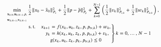
In the MHE the measurement noise is introduced as a new optimization variable and the measurement equation is added as an additional constraint. The full optimization problem now looks like this: image This change makes it possible for the user to decide, which measurements are enforced and which can be perturbed. A typical example would be to ensure that input “measurements” are completely trusted.

Simulator with disturbances¶

The newly introduced measurement noise and the existing process noise are now used within the simulator. With each call of Simulator.make_step values can be passed to obtain an imperfectly simulated and measured system..

Documentation¶

Release notes are now included in the documentation. They are autogenerated from the Github release notes which can be accessed via Rest API.
The release notes are appended with a section that includes a download link for the example files that were written for the respective versions.
Installation instructions now refer to these download links. This solves #62 .
Added new section Example gallery, explaining the supplied examples in do-mpc in Jupyter Notebooks (rendered on readthedocs)
Added new section Background with various articles explaining the mathematics behind do-mpc.
Parameter collocation_ni in MPC/MHE is now explained more clearly.

Minor changes¶

Renamed model.setup_model() -> model.setup()in all examples. This adresses #38
opt_p_num and opt_x_num for MHE/MPC are now instance properties instead of class attributes. They still appear in the documentation and can be used as before. Having them as class attributes can lead to problems when multiple classes are live during the same session.

Example files¶

Please download the example files for release do-mpc v4.0.0 here.

do-mpc v4.0.0-beta3¶

Major changes¶

Data¶

New __getitem__ method to conveniently retrieve values from Data object (details here)
New MPCData class (which inherits form Data). This adds the prediction method, which can be used to query the optimal trajectories. Details here.

Both methods were previously (in a slightly different form) in the Graphics module. They are still used in this class but can also be convenient under different circumstances.

Graphics¶

The Graphics module is now initialized with a specific Data instance (e.g. mpc.data). Each Data class has their own Graphics class (if it is supposed to be displayed). Compared to the previous implementation, we now initialize all lines that are supposed to be plotted (and store them in pred_lines and result_lines). During runtime, the data on these lines is getting updated.

Added new structure class in do_mpc.tools. Used for tracking the new Graphics properties: pred_lines and result_lines.
The properties pred_lines and result_lines can be used to retrieve line instances with power indices. Line instances can be easily configured (linestyle, alpha, color etc.)

Process noise¶

Process noise can be added to rhs of Model class: link

This is solving issue #53 .

This change was necessary to allow for the more natural MHE formulation where the process noise is penalised in the cost function. The user can define for each state (vector) individually if this is intended or not.

As a consequence of this change I had to introduce the new variable w throughout do-mpc. For the MPC and simulator module this is without effect.

The main difference is here

Remark: The change also allows to estimate parameters that change over time (e.g. environmental influences). Our regular estimated parameters are constant over the entire MHE horizon, which is not always valid. To estimate varying parameters, they should be defined as states with unknown dynamics. Concretely, their RHS is zero (for ODEs) and they have a high process noise.

Symbolic variables for MHE weighting matrices¶

As originally intended, it is now possible to have symbolic matrices as MHE tuning factors. The result of this change can be seen in the rotating_oscillating_masses example.

The symbolic variables are defined in the do-mpc Model where typically, you want to have P_x and P_p as parameters and P_y and P_w as time-varying parameters. Example of their definition.

and here they are used.

The purpose of using symbolic weighting is of course to update them at each iteration. Since they are parameters and time-varying parameters respectively, this is done with the set_p_fun and set_tvp_fun method of the MHE: link

Note that in the example above, we don’t actually need varying weighting matrices and the returned values are in fact constant. This can be seen as a proof of concept.

This change had some other implications. Most notably, having additional parameters interferes with the multi-stage robust MPC module. Where we previously had to pass a number of scenarios for each defined parameter. Since parameters for the MHE are irrelevant for MPC the API for the call set_uncertainty_values has changed: link

The new API is fully backwards compatible. However, it is much more intuitive now. The function is called with keyword arguments, where each keyword refers to one uncertain parameter (note that we can ignore the parameters that are irrelevant). In practice this looks something like this

Example files¶

Please download the example files for release do-mpc v4.0.0-beta3 here.

do-mpc v4.0.0-beta2¶

Error in release. Immediately replaced with beta3.

do-mpc v4.0.0-beta1¶

Major changes¶

We are now explicitly pointing out attributes of the Model such as states, inputs, etc. These should be used to obtain these attributes and replace the previous get_variables method which is now depreciated. The Model also supports a __get_variable__ call now to conveniently select items.
setup_model is replaced by setup to be more consistent with other setup methods. The old method is still available and shows a depreciation warning.
The MHE now supports the set_default_objective method.

Bug fixes¶

The MHE formulation had an error in the make_step method. We used the wrong time step from the previous solution to compute the arrival cost.

Other changes¶

Spelling in documentation
New guide about installing HSL linear solver
Credits in documentation

Example files¶

Please download the example files for release do-mpc v4.0.0-beta1 here.

do-mpc v4.0.0-beta¶

do-mpc has undergone a massive overhaul and comes with a completely new interface, new features and a comprehensive documentation.

Please note that previously written code is not compatible with do-mpc 4.0.0. If you want to continue working with older code please use version 3.0.0.

This is the beta release of version 4.0.0. We expect minor modifications and bug fixes in the near future.

Please see our documentation on our new project homepage www.do-mpc.com for a full list of features.

Release notes¶

v4.2.0¶

Major changes¶

MX support¶

Minor changes¶

Bug fixes¶

v4.1.1¶

Major changes¶

Adapted time-varying parameters for MPC object¶

Documentation¶

do-mpc v4.1.0¶

Major changes¶

DAE support¶

Continuous time (orthogonal collocation)¶

Discrete time¶

Constraints with MPC / MHE with orthogonal collocation¶

Terminal bounds for MPC¶

Minor changes¶

Documentation¶

Example files¶

do-mpc v4.0.0¶

Major changes¶

New properties for Simulator, Estimator and MPC¶

Set initial values¶

Obtain the current values of the iterated variables¶

Measurement noise¶

Simulator with disturbances¶

Documentation¶

Minor changes¶

Example files¶

do-mpc v4.0.0-beta3¶

Major changes¶

Data¶

Graphics¶

Process noise¶

Symbolic variables for MHE weighting matrices¶

Example files¶

do-mpc v4.0.0-beta2¶

do-mpc v4.0.0-beta1¶

Major changes¶

Bug fixes¶

Other changes¶

Example files¶

do-mpc v4.0.0-beta¶

Example files¶

do-mpc v3.0.0¶

Main modifications¶

do-mpc v2.0.0¶

do-mpc version 1.0.0¶