Continuous stirred tank reactor (CSTR) - LQR

In this Jupyter Notebook we illustrate the example CSTR. We design a Linear Quadratic Regulator(LQR) to regulate CSTR.

Open an interactive online Jupyter Notebook with this content on Binder:

The example consists of the three modules template_model.py, which describes the system model, template_lqr.py, which defines the settings for the control and template_simulator.py, which sets the parameters for the simulator. The modules are used in main.py for the closed-loop execution of the controller. The file post_processing.py is used for the visualization of the closed-loop control run.

In the following the different parts are presented. But first, we start by importing basic modules and do-mpc.

import numpy as np
import sys
from casadi import *
from casadi.tools import *
import matplotlib.pyplot as plt
import pdb

# Add do_mpc to path. This is not necessary if it was installed via pip
import os
rel_do_mpc_path = os.path.join('..','..','..')
sys.path.append(rel_do_mpc_path)

# Import do_mpc package:
import do_mpc
from do_mpc.tools import Timer
import pickle
import time

Model

In the following we will present the configuration, setup and connection between these blocks, starting with the model. The considered model of the CSTR is continuous and has 4 states and 2 control inputs. The model is initiated by:

model_type = 'continuous' # either 'discrete' or 'continuous'
model = do_mpc.model.Model(model_type)

States and control inputs

The four states are concentration of reactant A (\(C_{\text{A}}\)), the concentration of reactant B (\(C_{\text{B}}\)), the temperature inside the reactor (\(T_{\text{R}}\)) and the temperature of the cooling jacket (\(T_{\text{J}}\)):

# States struct (optimization variables):
C_a = model.set_variable(var_type='_x', var_name='C_a', shape=(1,1))
C_b = model.set_variable(var_type='_x', var_name='C_b', shape=(1,1))
T_R = model.set_variable(var_type='_x', var_name='T_R', shape=(1,1))
T_J = model.set_variable(var_type='_x', var_name='T_J', shape=(1,1))

The control inputs are the feed \(Fr\) and the heat removal by the jacket \(Q_J\):

# Input struct (optimization variables):
Fr = model.set_variable(var_type='_u', var_name='Fr')
Q_J = model.set_variable(var_type='_u', var_name='Q_J')

ODE and parameters

The system model is described by the ordinary differential equation:

\begin{align} \dot{C}_{\text{A}} &= \frac{Fr}{V} \cdot (C_{\text{A}_{in}} - C_{\text{A}}) - r_1, \\ \dot{C}_{\text{B}} &= -\frac{Fr}{V} \cdot C_{\text{B}} + r_1 - r_2, \\ \dot{T}_{\text{R}} &= \frac{Fr}{V} \cdot (T_{\text{in}-T_{\text{R}}}) -\frac{k \cdot A \cdot (T_{\text{R}}-T_{\text{J}})}{\rho \cdot c_{\text{p}} \cdot V} +\frac{\Delta H_{\text{R,1}}\cdot (-r_1)+\Delta H_{\text{R,2}}\cdot (-r_2)}{\rho \cdot c_{\text{p}}}, \\ \dot{T}_{\text{J}} &= \frac{-Q_{\text{J}} + k \cdot A \cdot (T_{\text{R}}-T_{\text{J}})}{m_j \cdot C_{p,J}}, \\ \end{align}

where

\begin{align} r_1 &= k_{0,1}\cdot\exp\left(\frac{-E_{\text{R,1}}}{T_{\text{R}}}\right)\cdot C_{\text{A}} \\ r_2 &= k_{0,2}\cdot\exp\left(\frac{-E_{\text{R,2}}}{T_{\text{R}}}\right)\cdot C_{\text{B}}\\ \end{align}

# Certain parameters
K0_1 = 2.145e10      # [min^-1]
K0_2 = 2.145e10      # [min^-1]
E_R_1 = 9758.3       # [K]
E_R_2 = 9758.3       # [K]
delH_R_1 = -4200     # [kJ/kmol]
del_H_R_2 = -11000   # [kJ/kmol]
T_in = 387.05        # [K]
rho = 934.2          # [kg/m^3]
cp = 3.01            # [kJ/m^3.K]
cp_J = 2             # [kJ/m^3.K]
m_j = 5              # [kg]
kA = 14.448          # [kJ/min.K]
C_ain = 5.1          # [kmol/m^3]
V = 0.01             # [m^3]

In the next step, we formulate the \(r_i\)-s:

# Auxiliary terms
r_1 = K0_1 * exp((-E_R_1)/((T_R)))*C_a
r_2 = K0_2 * exp((-E_R_2)/((T_R)))*C_b

WIth the help ot the \(k_i\)-s and other available parameters we can define the ODEs:

# Differential equations
model.set_rhs('C_a', (Fr/V)*(C_ain-C_a)-r_1)
model.set_rhs('C_b', -(Fr/V)*C_b + r_1 - r_2)
model.set_rhs('T_R', (Fr/V)*(T_in-T_R)-(kA/(rho*cp*V))*(T_R-T_J)+(1/(rho*cp))*((delH_R_1*(-r_1))+(del_H_R_2*(-r_2))))
model.set_rhs('T_J', (1/(m_j*cp_J))*(-Q_J+kA*(T_R-T_J)))

Finally, the model setup is completed:

# Build the model
model.setup()

To design a LQR, we need a discrete Linear Time Invariant (LTI) system. In the following blocks of code, we will obtain such a model. Firstly, we will linearize a non-linear model around equilibrium point.

# Steady state values
F_ss = 0.002365    # [m^3/min]
Q_ss = 18.5583     # [kJ/min]

C_ass = 1.6329     # [kmol/m^3]
C_bss = 1.1101     # [kmolm^3]
T_Rss = 398.6581   # [K]
T_Jss = 397.3736   # [K]

uss = np.array([[F_ss],[Q_ss]])
xss = np.array([[C_ass],[C_bss],[T_Rss],[T_Jss]])

# Linearize the non-linear model
linearmodel = do_mpc.model.linearize(model, xss, uss)

Now we dicretize the continuous LTI model with sampling time \(t_\text{step} = 0.5\) .

t_step = 0.5
model_dc = linearmodel.discretize(t_step, conv_method = 'zoh') # ['zoh','foh','bilinear','euler','backward_diff','impulse']

d:\Study_Materials\student_job\research_assistant\work_files\do_mpc_git\do-mpc\documentation\source\example_gallery\..\..\..\do_mpc\model\_linearmodel.py:296: UserWarning: sampling time is 0.5
  warnings.warn('sampling time is {}'.format(t_step))

Controller

Now, we design Linear Quadratic Regulator for the above configured model. First, we create an instance of the class.

# Initialize the controller
lqr = do_mpc.controller.LQR(model_dc)

We choose the prediction horizon n_horizon = 10, the time step t_step = 0.5s second.

# Initialize parameters
setup_lqr = {'t_step':t_step}
lqr.set_param(**setup_lqr)

Objective

The goal of CSTR is to drive the states to the desired set points.

Inputs:

Input	SetPoint
\(Fr_{\text{ref}}\)	\(0.002365 \frac{m^3}{min}\)
\(Q_{\text{J,ref}}\)	\(18.5583 \frac{kJ}{min}\)

States:

States	SetPoint
\(C_{\text{A,ref}}\)	\(1.6329 \frac{kmol}{m^3}\)
\(C_{\text{B,ref}}\)	\(1.1101 \frac{kmol}{m^3}\)
\(T_{\text{R,ref}}\)	\(398.6581 K\)
\(T_{\text{J,ref}}\)	\(397.3736 K\)

# Set objective
Q = 10*np.array([[1,0,0,0],[0,1,0,0],[0,0,0.01,0],[0,0,0,0.01]])
R = np.array([[1e-1,0],[0,1e-5]])

lqr.set_objective(Q=Q, R=R)

Now we run the LQR with the rated input. In order to do so, we set the cost matrix for the rated input as below:

Rdelu = np.array([[1e8,0],[0,1]])
lqr.set_rterm(delR = Rdelu)

Finally, LQR setup is completed

# set up lqr
lqr.setup()

d:\Study_Materials\student_job\research_assistant\work_files\do_mpc_git\do-mpc\documentation\source\example_gallery\..\..\..\do_mpc\controller\_lqr.py:478: UserWarning: discrete infinite horizon gain will be computed since prediction horizon is set to default value 0
  warnings.warn('discrete infinite horizon gain will be computed since prediction horizon is set to default value 0')

Estimator

We assume, that all states can be directly measured (state-feedback):

estimator = do_mpc.estimator.StateFeedback(model)

Simulator

To create a simulator in order to run the LQR in a closed-loop, we create an instance of the do-mpc simulator which is based on the non-linear model:

simulator = do_mpc.simulator.Simulator(model)

For the simulation, we use the same time step t_step as for the optimizer:

params_simulator = {
    'integration_tool': 'cvodes',
    'abstol': 1e-10,
    'reltol': 1e-10,
    't_step': t_step
}

simulator.set_param(**params_simulator)

To finish the configuration of the simulator, call:

simulator.setup()

Closed-loop simulation

For the simulation of the LQR configured for the CSTR, we inspect the file main.py. We define the initial state of the system and set it for all parts of the closed-loop configuration. Furthermore, we set the desired destination for the states and input.

# Set the initial state of simulator:
C_a0 = 0
C_b0 = 0
T_R0 = 387.05
T_J0 = 387.05

x0 = np.array([C_a0, C_b0, T_R0, T_J0]).reshape(-1,1)

simulator.x0 = x0

lqr.set_setpoint(xss=xss,uss=uss)

Now, we simulate the closed-loop for 100 steps:

#Run LQR main loop:
sim_time = 100
for k in range(sim_time):
    u0 = lqr.make_step(x0)
    y_next = simulator.make_step(u0)
    x0 = y_next

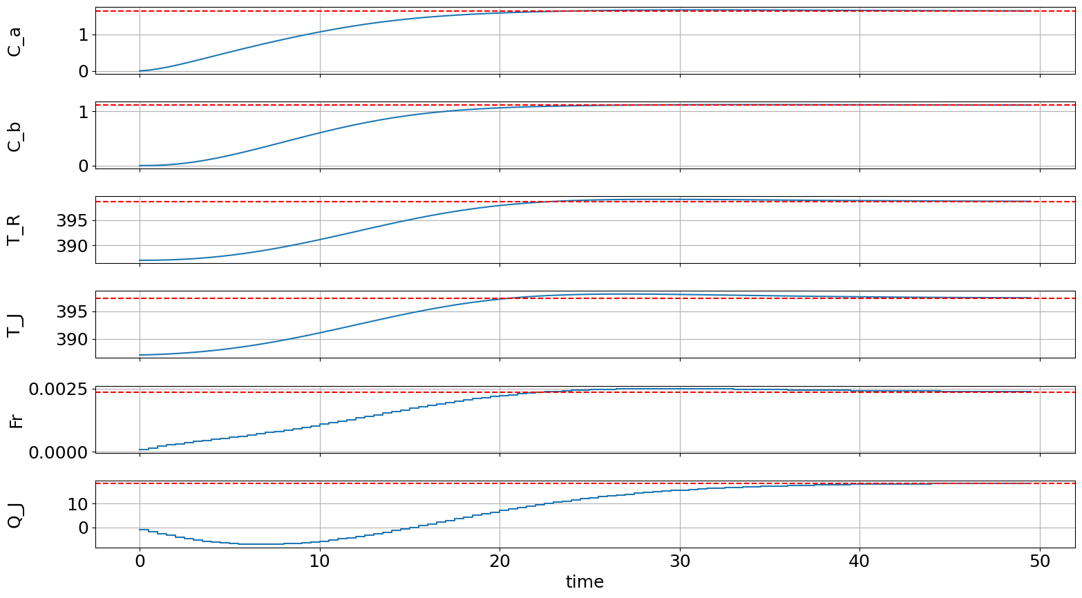
Plotting

Now we plot the results obtained in the closed loop simulation.

from matplotlib import rcParams
rcParams['axes.grid'] = True
rcParams['font.size'] = 18

fig, ax, graphics = do_mpc.graphics.default_plot(simulator.data, figsize=(16,9))
graphics.plot_results()
graphics.reset_axes()
ax[0].axhline(y=C_ass,xmin=0,xmax=sim_time*t_step,color='r',linestyle='dashed')
ax[1].axhline(y=C_bss,xmin=0,xmax=sim_time*t_step,color='r',linestyle='dashed')
ax[2].axhline(y=T_Rss,xmin=0,xmax=sim_time*t_step,color='r',linestyle='dashed')
ax[3].axhline(y=T_Jss,xmin=0,xmax=sim_time*t_step,color='r',linestyle='dashed')
ax[4].axhline(y=F_ss,xmin=0,xmax=sim_time*t_step,color='r',linestyle='dashed')
ax[5].axhline(y=Q_ss,xmin=0,xmax=sim_time*t_step,color='r',linestyle='dashed')
plt.show()