Efficient data generation and handling with do-mpc

This notebook was used in our video tutorial on data generation and handling with do-mpc.

We start by importing basic modules and do-mpc.

import numpy as np
import sys
from casadi import *
import os
import time

# Add do_mpc to path. This is not necessary if it was installed via pip
import os
rel_do_mpc_path = os.path.join('..','..','..')
sys.path.append(rel_do_mpc_path)

# Import do_mpc package:
import do_mpc

import matplotlib.pyplot as plt

import pandas as pd

Toy example

Step 1: Create the sampling_plan with the SamplingPlanner.

The planner is initiated and we set some (optional) parameters.

sp = do_mpc.sampling.SamplingPlanner()
sp.set_param(overwrite = True)
# This generates the directory, if it does not exist already.
sp.data_dir = './sampling_test/'

We then introduce new variables to the SamplingPlanner which will later jointly define a sampling case. Think of header rows in a table (see figure above).

These variables can themselves be sampled from a generating function or we add user defined cases one by one. If we want to sample variables to define the sampling case, we need to pass a sample generating function as shown below:

sp.set_sampling_var('alpha', np.random.randn)
sp.set_sampling_var('beta', lambda: np.random.randint(0,5))

In this example we have two variables alpha and beta. We have:

\[\alpha \sim \mathcal{N}(\mu,\sigma)\]

and

\[\beta\sim \mathcal{U}([0,5])\]

Having defined generating functions for all of our variables, we can now generate a sampling plan with an arbitrary amount of cases:

SamplingPlanner.gen_sampling_plan(n_samples)

plan = sp.gen_sampling_plan(n_samples=10)

We can inspect the plan conveniently by converting it to a pandas DataFrame. Natively, the plan is a list of dictionaries.

pd.DataFrame(plan)

	alpha	beta	id
0	0.105326	0	000
1	0.784304	2	001
2	0.257489	1	002
3	1.552975	1	003
4	0.053229	3	004
5	1.041070	4	005
6	0.473513	0	006
7	0.917850	3	007
8	0.984259	0	008
9	0.715357	0	009

If we do not wish to automatically generate a sampling plan, we can also add sampling cases one by one with:

plan = sp.add_sampling_case(alpha=1, beta=-0.5)
print(plan[-1])

{'alpha': 1, 'beta': -0.5, 'id': '010'}

Typically, we finish the process of generating the sampling plan by saving it to the disc. This is simply done with:

sp.export(sampling_plan_name)

The save directory was already set with sp.data_dir = ....

Step 2: Create the Sampler object by providing the sampling_plan:

sampler = do_mpc.sampling.Sampler(plan)
sampler.set_param(overwrite = True)

Most important settting of the sampler is the sample_function. This function takes as arguments previously the defined sampling_var (from the configuration of the SamplingPlanner).

It this example, we create a dummy sampling generating function, where:

\[f(\alpha,\beta) = \alpha\cdot\beta\]

def sample_function(alpha, beta):
    time.sleep(0.1)
    return alpha*beta

sampler.set_sample_function(sample_function)

Before we sample, we want to set the directory for the created files and a name:

sampler.data_dir = './sampling_test/'
sampler.set_param(sample_name = 'dummy_sample')

Now we can actually create all the samples:

sampler.sample_data()

Progress: |██████████████████████████████████████████████████| 100.0% Complete

The sampler will now create the sampling results as a new file for each result and store them in a subfolder with the same name as the sampling_plan:

ls = os.listdir('./sampling_test/')
ls.sort()
ls

['dummy_sample_000.pkl',
 'dummy_sample_001.pkl',
 'dummy_sample_002.pkl',
 'dummy_sample_003.pkl',
 'dummy_sample_004.pkl',
 'dummy_sample_005.pkl',
 'dummy_sample_006.pkl',
 'dummy_sample_007.pkl',
 'dummy_sample_008.pkl',
 'dummy_sample_009.pkl',
 'dummy_sample_010.pkl',
 'dummy_sample_011.pkl',
 'dummy_sample_012.pkl']

Step 3: Process data in the data handler class.

The first step is to initiate the class with the sampling_plan:

dh = do_mpc.sampling.DataHandler(plan)

We then need to point out where the data is stored and how the samples are called:

dh.data_dir = './sampling_test/'
dh.set_param(sample_name = 'dummy_sample')

Next, we define the post-processing functions. For this toy example we do some “dummy” post-processing and request to compute two results:

dh.set_post_processing('res_1', lambda x: x)
dh.set_post_processing('res_2', lambda x: x**2)

The interface of DataHandler.set_post_processing requires a name that we will see again later and a function that processes the output of the previously defined sample_function.

We can now obtain obtain processed data from the DataHandler in two ways. Note that we convert the returned list of dictionaries directly to a DataFrame for a better visualization.

1. Indexing:

pd.DataFrame(dh[:3])

	alpha	beta	id	res_1	res_2
0	0.105326	0	000	0.000000	0.000000
1	0.784304	2	001	1.568608	2.460532
2	0.257489	1	002	0.257489	0.066301

Or we use a more complex filter with the DataHandler.filter method. This method requires either an input or an output filter in the form of a function.

Let’s retrieve all samples, where \(\alpha < 0\):

pd.DataFrame(dh.filter(input_filter = lambda alpha: alpha<0))

Or we can filter by outputs, e.g. with:

pd.DataFrame(dh.filter(output_filter = lambda res_2: res_2>10))

	alpha	beta	id	res_1	res_2
0	1.04107	4	005	4.164281	17.341236

Sampling closed-loop trajectories

A more reasonable use-case in the scope of do-mpc is to sample closed-loop trajectories of a dynamical system with a (MPC) controller.

The approach is almost identical to our toy example above. The main difference lies in the sample_function that is passed to the Sampler and the post_processing in the DataHandler.

In the presented example, we will sample the oscillating mass system which is part of the do-mpc example library.

sys.path.append('../../../examples/oscillating_masses_discrete/')
from template_model import template_model
from template_mpc import template_mpc
from template_simulator import template_simulator

Step 1: Create the sampling plan with the SamplingPlanner

We want to generate various closed-loop trajectories of the system starting from random initial states, hence we design the SamplingPlanner as follows:

# Initialize sampling planner
sp = do_mpc.sampling.SamplingPlanner()
sp.set_param(overwrite=True)

# Sample random feasible initial states
def gen_initial_states():

    x0 = np.random.uniform(-3*np.ones((4,1)),3*np.ones((4,1)))

    return x0

# Add sampling variable including the corresponding evaluation function
sp.set_sampling_var('X0', gen_initial_states)

This implementation is sufficient to generate the sampling plan:

plan = sp.gen_sampling_plan(n_samples=9)

Since we want to run the system in the closed-loop in our sample function, we need to load the corresponding configuration:

model = template_model()
mpc = template_mpc(model)
estimator = do_mpc.estimator.StateFeedback(model)
simulator = template_simulator(model)

We can now define the sampling function:

def run_closed_loop(X0):
    mpc.reset_history()
    simulator.reset_history()
    estimator.reset_history()

    # set initial values and guess
    x0 = X0
    mpc.x0 = x0
    simulator.x0 = x0
    estimator.x0 = x0

    mpc.set_initial_guess()

    # run the closed loop for 150 steps
    for k in range(100):
        u0 = mpc.make_step(x0)
        y_next = simulator.make_step(u0)
        x0 = estimator.make_step(y_next)

    # we return the complete data structure that we have obtained during the closed-loop run
    return simulator.data

Now we have all the ingredients to make our sampler:

%%capture
# Initialize sampler with generated plan
sampler = do_mpc.sampling.Sampler(plan)
# Set directory to store the results:
sampler.data_dir = './sampling_closed_loop/'
sampler.set_param(overwrite=True)

# Set the sampling function
sampler.set_sample_function(run_closed_loop)

# Generate the data
sampler.sample_data()

Step 3: Process data in the data handler class. The first step is to initiate the class with the sampling_plan:

# Initialize DataHandler
dh = do_mpc.sampling.DataHandler(plan)
dh.data_dir = './sampling_closed_loop/'

In this case, we are interested in the states and the inputs of all trajectories. We define the following post processing functions:

dh.set_post_processing('input', lambda data: data['_u', 'u'])
dh.set_post_processing('state', lambda data: data['_x', 'x'])

To retrieve all post-processed data from the datahandler we use slicing. The result is stored in res.

res = dh[:]

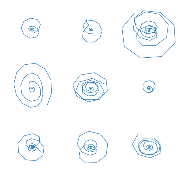
To inspect the sampled closed-loop trajectories, we create an array of plots where in each plot \(x_2\) is plotted over \(x_1\). This shows the different behavior, based on the sampled initial conditions:

n_res = min(len(res),80)

n_row = int(np.ceil(np.sqrt(n_res)))
n_col = int(np.ceil(n_res/n_row))


fig, ax = plt.subplots(n_row, n_col, sharex=True, sharey=True, figsize=(8,8))
for i, res_i in enumerate(res):
    ax[i//n_col, np.mod(i,n_col)].plot(res_i['state'][:,1],res_i['state'][:,0])

for i in range(ax.size):
    ax[i//n_col, np.mod(i,n_col)].axis('off')



fig.tight_layout(pad=0)