
Industrial polymerization reactor#
In this Jupyter Notebook we illustrate the example industrial_poly.
Open an interactive online Jupyter Notebook with this content on Binder:
![]()
The example consists of the three modules template_model.py, which describes the system model, template_mpc.py, which defines the settings for the control and template_simulator.py, which sets the parameters for the simulator. The modules are used in main.py for the closed-loop execution of the controller.
In the following the different parts are presented. But first, we start by importing basic modules and do-mpc.
[29]:
import numpy as np
import matplotlib.pyplot as plt
import sys
from casadi import *

# Add do_mpc to path. This is not necessary if it was installed via pip
import os
rel_do_mpc_path = os.path.join('..','..','..')
sys.path.append(rel_do_mpc_path)

# Import do_mpc package:
import do_mpc
Model#
In the following we will present the configuration, setup and connection between these blocks, starting with the model. The considered model of the industrial reactor is continuous and has 10 states and 3 control inputs. The model is initiated by:
[2]:
model_type = 'continuous' # either 'discrete' or 'continuous'
model = do_mpc.model.Model(model_type)
System description#
The system consists of a reactor into which nonomer is fed. The monomerturns into a polymer via a very exothermic chemical reaction. The reactor is equipped with a jacket and with an External Heat Exchanger(EHE) that can both be used to control the temperature inside the reactor. A schematic representation of the system is presented below:

The process is modeled by a set of 8 ordinary differential equations (ODEs):
\begin{align} \dot{m}_{\text{W}} &= \ \dot{m}_{\text{F}}\, \omega_{\text{W,F}} \\ \dot{m}_{\text{A}} &= \ \dot{m}_{\text{F}} \omega_{\text{A,F}}-k_{\text{R1}}\, m_{\text{A,R}}-k_{\text{R2}}\, m_{\text{AWT}}\, m_{\text{A}}/m_{\text{ges}} , \\ \dot{m}_{\text{P}} &= \ k_{\text{R1}} \, m_{\text{A,R}}+p_{1}\, k_{\text{R2}}\, m_{\text{AWT}}\, m_{\text{A}}/ m_{\text{ges}}, \\ \dot{T}_{\text{R}} &= \ 1/(c_{\text{p,R}} m_{\text{ges}})\; [\dot{m}_{\text{F}} \; c_{\text{p,F}}\left(T_{\text{F}}-T_{\text{R}}\right) +\Delta H_{\text{R}} k_{\text{R1}} m_{\text{A,R}}-k_{\text{K}} A\left(T_{\text{R}}-T_{\text{S}}\right) \\ &- \dot{m}_{\text{AWT}} \,c_{\text{p,R}}\left(T_{\text{R}}-T_{\text{EK}}\right)],\notag\\ \dot{T}_{S} &= 1/(c_{\text{p,S}} m_{\text{S}}) \;[k_{\text{K}} A\left(T_{\text{R}}-T_{\text{S}}\right)-k_{\text{K}} A\left(T_{\text{S}}-T_{\text{M}}\right)], \notag\\ \dot{T}_{\text{M}} &= 1/(c_{\text{p,W}} m_{\text{M,KW}})\;[\dot{m}_{\text{M,KW}}\, c_{\text{p,W}}\left(T_{\text{M}}^{\text{IN}}-T_{\text{M}}\right) \\ &+ k_{\text{K}} A\left(T_{\text{S}}-T_{\text{M}}\right)]+k_{\text{K}} A\left(T_{\text{S}}-T_{\text{M}}\right)], \\ \dot{T}_{\text{EK}}&= 1/(c_{\text{p,R}} m_{\text{AWT}})\;[\dot{m}_{\text{AWT}} c_{\text{p,W}}\left(T_{\text{R}}-T_{\text{EK}}\right)-\alpha\left(T_{\text{EK}}-T_{\text{AWT}}\right) \\ &+ k_{\text{R2}}\, m_{\text{A}}\, m_{\text{AWT}}\Delta H_{\text{R}}/m_{\text{ges}}], \notag\\ \dot{T}_{\text{AWT}} &= [\dot{m}_{\text{AWT,KW}} \,c_{\text{p,W}}\,(T_{\text{AWT}}^{\text{IN}}-T_{\text{AWT}})-\alpha\left(T_{\text{AWT}}-T_{\text{EK}}\right)]/(c_{\text{p,W}} m_{\text{AWT,KW}}), \end{align}
where
\begin{align} U &= m_{\text{P}}/(m_{\text{A}}+m_{\text{P}}), \\ m_{\text{ges}} &= \ m_{\text{W}}+m_{\text{A}}+m_{\text{P}}, \\ k_{\text{R1}} &= \ k_{0} e^{\frac{-E_{a}}{R (T_{\text{R}}+273.15)}}\left(k_{\text{U1}}\left(1-U\right)+k_{\text{U2}} U\right), \\ k_{\text{R2}} &= \ k_{0} e^{\frac{-E_{a}}{R (T_{\text{EK}}+273.15)}}\left(k_{\text{U1}}\left(1-U\right)+k_{\text{U2}} U\right), \\ k_{\text{K}} &= (m_{\text{W}}k_{\text{WS}}+m_{\text{A}}k_{\text{AS}}+m_{\text{P}}k_{\text{PS}})/m_{\text{ges}},\\ m_{\text{A,R}} &= m_\text{A}-m_\text{A} m_{\text{AWT}}/m_{\text{ges}}. \end{align}
The model includes mass balances for the water, monomer and product hold-ups (\(m_\text{W}\), \(m_\text{A}\), \(m_\text{P}\)) and energy balances for the reactor (\(T_\text{R}\)), the vessel (\(T_\text{S}\)), the jacket (\(T_\text{M}\)), the mixture in the external heat exchanger (\(T_{\text{EK}}\)) and the coolant leaving the external heat exchanger (\(T_{\text{AWT}}\)). The variable \(U\) denotes the polymer-monomer ratio in the reactor, \(m_{\text{ges}}\) represents the total mass, \(k_{\text{R1}}\) is the reaction rate inside the reactor and \(k_{\text{R2}}\) is the reaction rate in the external heat exchanger. The total heat transfer coefficient of the mixture inside the reactor is denoted as \(k_{\text{K}}\) and \(m_{\text{A,R}}\) represents the current amount of monomer inside the reactor.
The available control inputs are the feed flow \(\dot{m}_{\text{F}}\), the coolant temperature at the inlet of the jacket \(T^{\text{IN}}_{\text{M}}\) and the coolant temperature at the inlet of the external heat exchanger \(T^{\text{IN}}_{\text{AWT}}\).
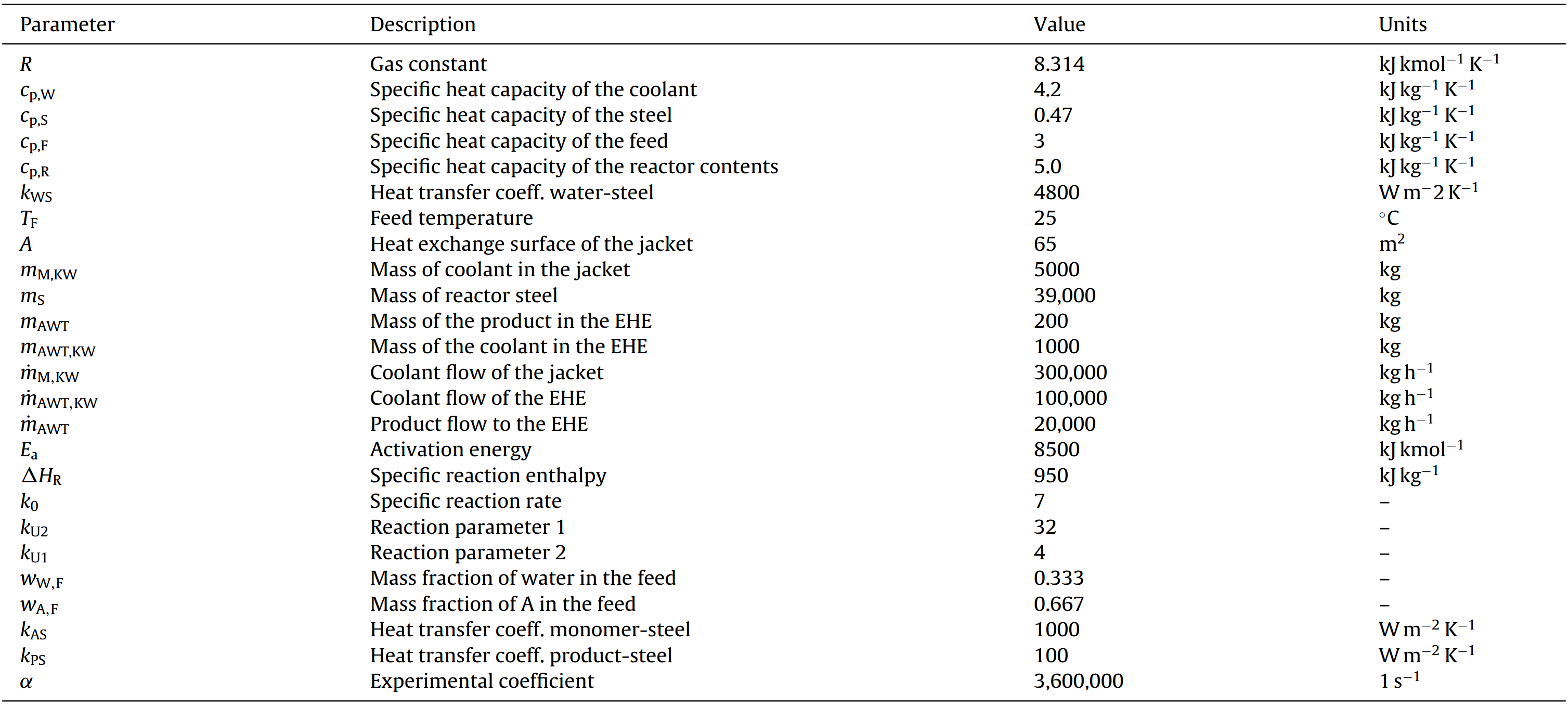
An overview of the parameters are listed below:
Implementation#
First, we set the certain parameters:
[3]:
# Certain parameters
R           = 8.314                 #gas constant
T_F         = 25 + 273.15   #feed temperature
E_a         = 8500.0                #activation energy
delH_R      = 950.0*1.00    #sp reaction enthalpy
A_tank      = 65.0                  #area heat exchanger surface jacket 65

k_0         = 7.0*1.00              #sp reaction rate
k_U2        = 32.0                  #reaction parameter 1
k_U1        = 4.0                   #reaction parameter 2
w_WF        = .333                  #mass fraction water in feed
w_AF        = .667                  #mass fraction of A in feed

m_M_KW      = 5000.0                #mass of coolant in jacket
fm_M_KW     = 300000.0              #coolant flow in jacket 300000;
m_AWT_KW    = 1000.0                #mass of coolant in EHE
fm_AWT_KW   = 100000.0              #coolant flow in EHE
m_AWT       = 200.0                 #mass of product in EHE
fm_AWT      = 20000.0               #product flow in EHE
m_S         = 39000.0               #mass of reactor steel

c_pW        = 4.2                   #sp heat cap coolant
c_pS        = .47                   #sp heat cap steel
c_pF        = 3.0                   #sp heat cap feed
c_pR        = 5.0                   #sp heat cap reactor contents

k_WS        = 17280.0               #heat transfer coeff water-steel
k_AS        = 3600.0                #heat transfer coeff monomer-steel
k_PS        = 360.0                 #heat transfer coeff product-steel

alfa        = 5*20e4*3.6

p_1         = 1.0
and afterwards the uncertain parameters:
[4]:
# Uncertain parameters:
delH_R = model.set_variable('_p', 'delH_R')
k_0 =    model.set_variable('_p', 'k_0')
The 10 states of the control problem stem from the 8 ODEs, accum_monom models the amount that has been fed to the reactor via \(\dot{m}_\text{F}^{\text{acc}} = \dot{m}_{\text{F}}\) and T_adiab (\(T_{\text{adiab}}=\frac{\Delta H_{\text{R}}}{c_{\text{p,R}}} \frac{m_{\text{A}}}{m_{\text{ges}}} + T_{\text{R}}\), hence
\(\dot{T}_{\text{adiab}}=\frac{\Delta H_{\text{R}}}{m_{\text{ges}} c_{\text{p,R}}}\dot{m}_{\text{A}}- \left(\dot{m}_{\text{W}}+\dot{m}_{\text{A}}+\dot{m}_{\text{P}}\right)\left(\frac{m_{\text{A}} \Delta H_{\text{R}}}{m_{\text{ges}}^2c_{\text{p,R}}}\right)+\dot{T}_{\text{R}}\)) is a virtual variable that is important for safety aspects, as we will explain later. All states are created in do-mpc via:
[5]:
# States struct (optimization variables):
m_W =         model.set_variable('_x', 'm_W')
m_A =         model.set_variable('_x', 'm_A')
m_P =         model.set_variable('_x', 'm_P')
T_R =         model.set_variable('_x', 'T_R')
T_S =         model.set_variable('_x', 'T_S')
Tout_M =      model.set_variable('_x', 'Tout_M')
T_EK =        model.set_variable('_x', 'T_EK')
Tout_AWT =    model.set_variable('_x', 'Tout_AWT')
accum_monom = model.set_variable('_x', 'accum_monom')
T_adiab =     model.set_variable('_x', 'T_adiab')
and the control inputs via:
[6]:
# Input struct (optimization variables):
m_dot_f = model.set_variable('_u', 'm_dot_f')
T_in_M =  model.set_variable('_u', 'T_in_M')
T_in_EK = model.set_variable('_u', 'T_in_EK')
Before defining the ODE for each state variable, we create auxiliary terms:
[7]:
# algebraic equations
U_m    = m_P / (m_A + m_P)
m_ges  = m_W + m_A + m_P
k_R1   = k_0 * exp(- E_a/(R*T_R)) * ((k_U1 * (1 - U_m)) + (k_U2 * U_m))
k_R2   = k_0 * exp(- E_a/(R*T_EK))* ((k_U1 * (1 - U_m)) + (k_U2 * U_m))
k_K    = ((m_W / m_ges) * k_WS) + ((m_A/m_ges) * k_AS) + ((m_P/m_ges) * k_PS)
The auxiliary terms are used for the more readable definition of the ODEs:
[8]:
# Differential equations
dot_m_W = m_dot_f * w_WF
model.set_rhs('m_W', dot_m_W)
dot_m_A = (m_dot_f * w_AF) - (k_R1 * (m_A-((m_A*m_AWT)/(m_W+m_A+m_P)))) - (p_1 * k_R2 * (m_A/m_ges) * m_AWT)
model.set_rhs('m_A', dot_m_A)
dot_m_P = (k_R1 * (m_A-((m_A*m_AWT)/(m_W+m_A+m_P)))) + (p_1 * k_R2 * (m_A/m_ges) * m_AWT)
model.set_rhs('m_P', dot_m_P)

dot_T_R = 1./(c_pR * m_ges)   * ((m_dot_f * c_pF * (T_F - T_R)) - (k_K *A_tank* (T_R - T_S)) - (fm_AWT * c_pR * (T_R - T_EK)) + (delH_R * k_R1 * (m_A-((m_A*m_AWT)/(m_W+m_A+m_P)))))
model.set_rhs('T_R', dot_T_R)
model.set_rhs('T_S', 1./(c_pS * m_S)     * ((k_K *A_tank* (T_R - T_S)) - (k_K *A_tank* (T_S - Tout_M))))
model.set_rhs('Tout_M', 1./(c_pW * m_M_KW)  * ((fm_M_KW * c_pW * (T_in_M - Tout_M)) + (k_K *A_tank* (T_S - Tout_M))))
model.set_rhs('T_EK', 1./(c_pR * m_AWT)   * ((fm_AWT * c_pR * (T_R - T_EK)) - (alfa * (T_EK - Tout_AWT)) + (p_1 * k_R2 * (m_A/m_ges) * m_AWT * delH_R)))
model.set_rhs('Tout_AWT', 1./(c_pW * m_AWT_KW)* ((fm_AWT_KW * c_pW * (T_in_EK - Tout_AWT)) - (alfa * (Tout_AWT - T_EK))))
model.set_rhs('accum_monom', m_dot_f)
model.set_rhs('T_adiab', delH_R/(m_ges*c_pR)*dot_m_A-(dot_m_A+dot_m_W+dot_m_P)*(m_A*delH_R/(m_ges*m_ges*c_pR))+dot_T_R)
Finally, the model setup is completed:
[9]:
# Build the model
model.setup()
Controller#
Next, the model predictive controller is configured (in template_mpc.py). First, one member of the mpc class is generated with the prediction model defined above:
[10]:
mpc = do_mpc.controller.MPC(model)
Real processes are also subject to important safety constraints that are incorporated to account for possible failures of the equipment. In this case, the maximum temperature that the reactor would reach in the case of a cooling failure is constrained to be below \(109 ^\circ\)C. The temperature that the reactor would achieve in the case of a complete cooling failure is \(T_{\text{adiab}}\), hence it needs to stay beneath \(109 ^\circ\)C.
We choose the prediction horizon n_horizon, set the robust horizon n_robust to 1. The time step t_step is set to one second and parameters of the applied discretization scheme orthogonal collocation are as seen below:
[11]:
setup_mpc = {
    'n_horizon': 20,
    'n_robust': 1,
    'open_loop': 0,
    't_step': 50.0/3600.0,
    'state_discretization': 'collocation',
    'collocation_type': 'radau',
    'collocation_deg': 2,
    'collocation_ni': 2,
    'store_full_solution': True,
    # Use MA27 linear solver in ipopt for faster calculations:
    #'nlpsol_opts': {'ipopt.linear_solver': 'MA27'}
}

mpc.set_param(**setup_mpc)
Objective#
The goal of the economic NMPC controller is to produce \(20680~\text{kg}\) of \(m_{\text{P}}\) as fast as possible. Additionally, we add a penalty on input changes for all three control inputs, to obtain a smooth control performance.
[12]:
_x = model.x
mterm = - _x['m_P'] # terminal cost
lterm = - _x['m_P'] # stage cost

mpc.set_objective(mterm=mterm, lterm=lterm)

mpc.set_rterm(m_dot_f=0.002, T_in_M=0.004, T_in_EK=0.002) # penalty on control input changes
Constraints#
The temperature at which the polymerization reaction takes place strongly influences the properties of the resulting polymer. For this reason, the temperature of the reactor should be maintained in a range of \(\pm 2.0 ^\circ\)C around the desired reaction temperature \(T_{\text{set}}=90 ^\circ\)C in order to ensure that the produced polymer has the required properties.
The initial conditions and the bounds for all states are summarized in:
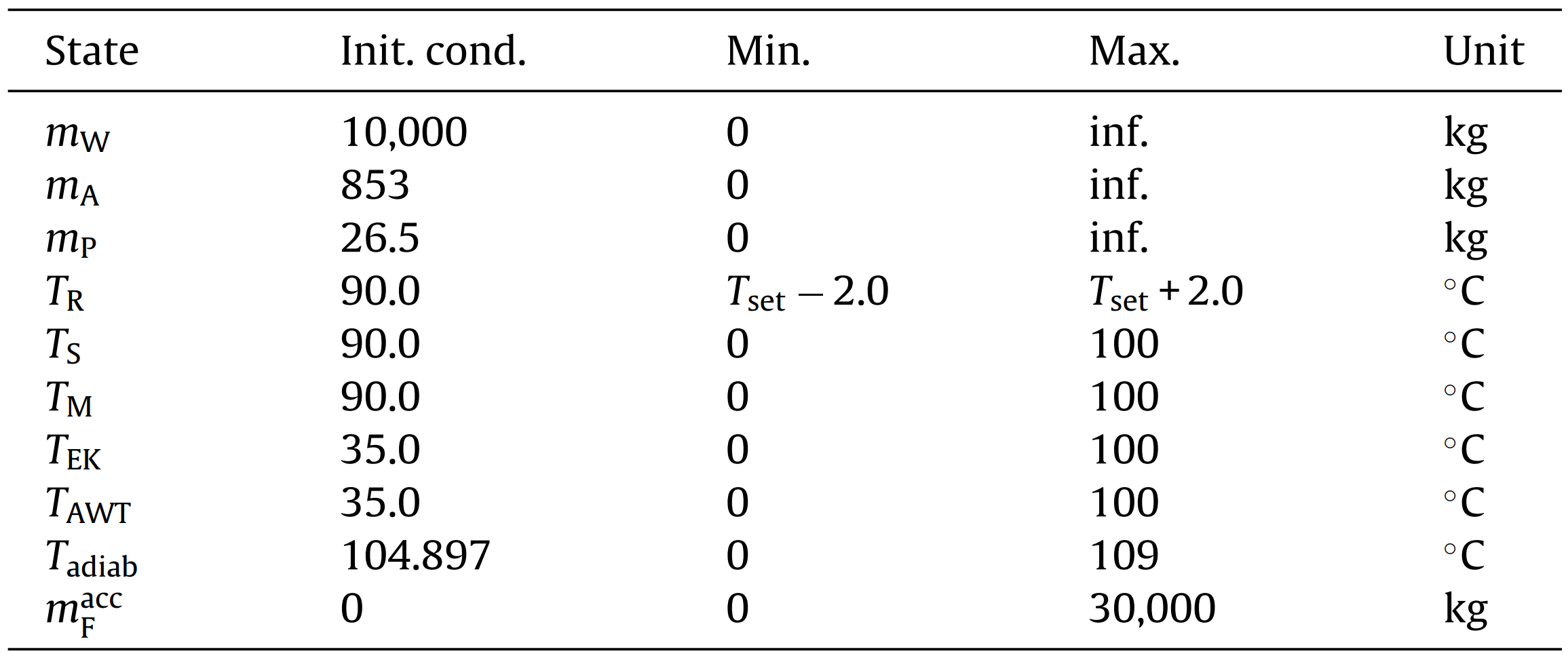
and set via:
[13]:
# auxiliary term
temp_range = 2.0

# lower bound states
mpc.bounds['lower','_x','m_W'] = 0.0
mpc.bounds['lower','_x','m_A'] = 0.0
mpc.bounds['lower','_x','m_P'] = 26.0

mpc.bounds['lower','_x','T_R'] = 363.15 - temp_range
mpc.bounds['lower','_x','T_S'] = 298.0
mpc.bounds['lower','_x','Tout_M'] = 298.0
mpc.bounds['lower','_x','T_EK'] = 288.0
mpc.bounds['lower','_x','Tout_AWT'] = 288.0
mpc.bounds['lower','_x','accum_monom'] = 0.0

# upper bound states
mpc.bounds['upper','_x','T_S'] = 400.0
mpc.bounds['upper','_x','Tout_M'] = 400.0
mpc.bounds['upper','_x','T_EK'] = 400.0
mpc.bounds['upper','_x','Tout_AWT'] = 400.0
mpc.bounds['upper','_x','accum_monom'] = 30000.0
mpc.bounds['upper','_x','T_adiab'] = 382.15
The upper bound of the reactor temperature is set via a soft-constraint:
[ ]:
mpc.set_nl_cons('T_R_UB', _x['T_R'], ub=363.15+temp_range, soft_constraint=True, penalty_term_cons=1e4)
The bounds of the inputsare summarized below:
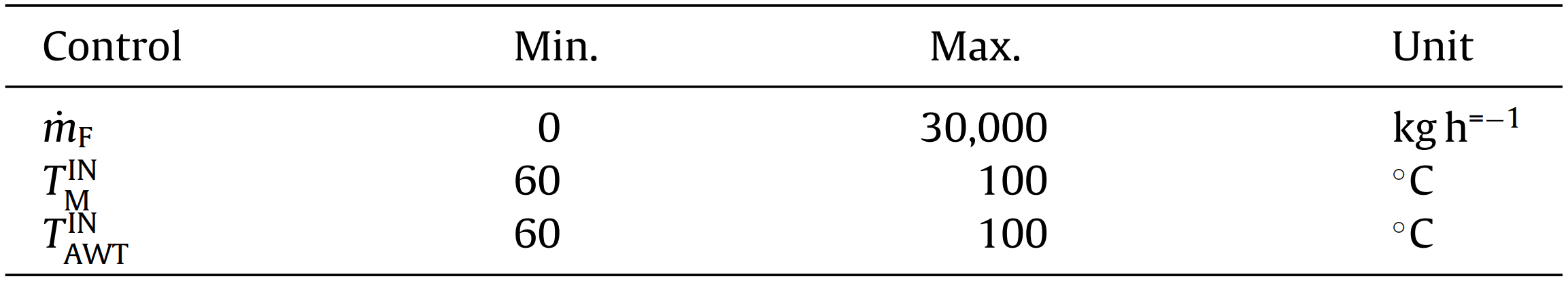
and set via:
[14]:
# lower bound inputs
mpc.bounds['lower','_u','m_dot_f'] = 0.0
mpc.bounds['lower','_u','T_in_M'] = 333.15
mpc.bounds['lower','_u','T_in_EK'] = 333.15

# upper bound inputs
mpc.bounds['upper','_u','m_dot_f'] = 3.0e4
mpc.bounds['upper','_u','T_in_M'] = 373.15
mpc.bounds['upper','_u','T_in_EK'] = 373.15
Scaling#
Because the magnitudes of the states and inputs are very different, the performance of the optimizer can be enhanced by properly scaling the states and inputs:
[15]:
# states
mpc.scaling['_x','m_W'] = 10
mpc.scaling['_x','m_A'] = 10
mpc.scaling['_x','m_P'] = 10
mpc.scaling['_x','accum_monom'] = 10

# control inputs
mpc.scaling['_u','m_dot_f'] = 100
Uncertain values#
In a real system, usually the model parameters cannot be determined exactly, what represents an important source of uncertainty. In this work, we consider that two of the most critical parameters of the model are not precisely known and vary with respect to their nominal value. In particular, we assume that the specific reaction enthalpy \(\Delta H_{\text{R}}\) and the specific reaction rate \(k_0\) are constant but uncertain, having values that can vary \(\pm 30 \%\) with respect to their nominal values
[16]:
delH_R_var = np.array([950.0, 950.0 * 1.30, 950.0 * 0.70])
k_0_var = np.array([7.0 * 1.00, 7.0 * 1.30, 7.0 * 0.70])

mpc.set_uncertainty_values(delH_R = delH_R_var, k_0 = k_0_var)
This means with n_robust=1, that 9 different scenarios are considered. The setup of the MPC controller is concluded by:
[17]:
mpc.setup()
Estimator#
We assume, that all states can be directly measured (state-feedback):
[18]:
estimator = do_mpc.estimator.StateFeedback(model)
Simulator#
To create a simulator in order to run the MPC in a closed-loop, we create an instance of the do-mpc simulator which is based on the same model:
[19]:
simulator = do_mpc.simulator.Simulator(model)
For the simulation, we use the same time step t_step as for the optimizer:
[20]:
params_simulator = {
    'integration_tool': 'cvodes',
    'abstol': 1e-10,
    'reltol': 1e-10,
    't_step': 50.0/3600.0
}

simulator.set_param(**params_simulator)
Realizations of uncertain parameters#
For the simulatiom, it is necessary to define the numerical realizations of the uncertain parameters in p_num. First, we get the structure of the uncertain parameters:
[21]:
p_num = simulator.get_p_template()
tvp_num = simulator.get_tvp_template()
We define a function which is called in each simulation step, which returns the current realizations of the parameters with respect to defined inputs (in this case t_now):
[22]:
# uncertain parameters
p_num['delH_R'] = 950 * np.random.uniform(0.75,1.25)
p_num['k_0'] = 7 * np.random.uniform(0.75*1.25)
def p_fun(t_now):
    return p_num
simulator.set_p_fun(p_fun)
By defining p_fun as above, the function will return a constant value for both uncertain parameters within a range of \(\pm 25\%\) of the nomimal value. To finish the configuration of the simulator, call:
[23]:
simulator.setup()
Closed-loop simulation#
For the simulation of the MPC configured for the CSTR, we inspect the file main.py. We define the initial state of the system and set it for all parts of the closed-loop configuration:
[24]:
# Set the initial state of the controller and simulator:
# assume nominal values of uncertain parameters as initial guess
delH_R_real = 950.0
c_pR = 5.0

# x0 is a property of the simulator - we obtain it and set values.
x0 = simulator.x0

x0['m_W'] = 10000.0
x0['m_A'] = 853.0
x0['m_P'] = 26.5

x0['T_R'] = 90.0 + 273.15
x0['T_S'] = 90.0 + 273.15
x0['Tout_M'] = 90.0 + 273.15
x0['T_EK'] = 35.0 + 273.15
x0['Tout_AWT'] = 35.0 + 273.15
x0['accum_monom'] = 300.0
x0['T_adiab'] = x0['m_A']*delH_R_real/((x0['m_W'] + x0['m_A'] + x0['m_P']) * c_pR) + x0['T_R']

mpc.x0 = x0
simulator.x0 = x0
estimator.x0 = x0

mpc.set_initial_guess()
Now, we simulate the closed-loop for 100 steps (and suppress the output of the cell with the magic command %%capture):
[25]:
%%capture
for k in range(100):
    u0 = mpc.make_step(x0)
    y_next = simulator.make_step(u0)
    x0 = estimator.make_step(y_next)
Animating the results#
To animate the results, we first configure the do-mpc graphics object, which is initiated with the respective data object:
[48]:
mpc_graphics = do_mpc.graphics.Graphics(mpc.data)
We quickly configure Matplotlib.
[49]:
from matplotlib import rcParams
rcParams['axes.grid'] = True
rcParams['font.size'] = 18
We then create a figure, configure which lines to plot on which axis and add labels.
[50]:
%%capture
fig, ax = plt.subplots(5, sharex=True, figsize=(16,12))
plt.ion()
# Configure plot:
mpc_graphics.add_line(var_type='_x', var_name='T_R', axis=ax[0])
mpc_graphics.add_line(var_type='_x', var_name='accum_monom', axis=ax[1])
mpc_graphics.add_line(var_type='_u', var_name='m_dot_f', axis=ax[2])
mpc_graphics.add_line(var_type='_u', var_name='T_in_M', axis=ax[3])
mpc_graphics.add_line(var_type='_u', var_name='T_in_EK', axis=ax[4])

ax[0].set_ylabel('T_R [K]')
ax[1].set_ylabel('acc. monom')
ax[2].set_ylabel('m_dot_f')
ax[3].set_ylabel('T_in_M [K]')
ax[4].set_ylabel('T_in_EK [K]')
ax[4].set_xlabel('time')

fig.align_ylabels()
After importing the necessary package:
[43]:
from matplotlib.animation import FuncAnimation, ImageMagickWriter
We obtain the animation with:
[51]:
def update(t_ind):
    print('Writing frame: {}.'.format(t_ind), end='\r')
    mpc_graphics.plot_results(t_ind=t_ind)
    mpc_graphics.plot_predictions(t_ind=t_ind)
    mpc_graphics.reset_axes()
    lines = mpc_graphics.result_lines.full
    return lines

n_steps = mpc.data['_time'].shape[0]


anim = FuncAnimation(fig, update, frames=n_steps, blit=True)

gif_writer = ImageMagickWriter(fps=5)
anim.save('anim_poly_batch.gif', writer=gif_writer)
Writing frame: 99.
We are displaying recorded values as solid lines and predicted trajectories as dashed lines. Multiple dashed lines exist for different realizations of the uncertain scenarios.
The most interesting behavior here can be seen in the state T_R, which has the upper bound:
[38]:
mpc.bounds['upper', '_x', 'T_R']
[38]:
DM(375.15)
Due to robust control, we are approaching this value but hold a certain distance as some possible trajectories predict a temperature increase. As the reaction finishes we can safely increase the temperature because a rapid temperature change due to uncertainy is impossible.