
Getting started: MPC#
In this Jupyter Notebook we illustrate the core functionalities of do-mpc.
Open an interactive online Jupyter Notebook with this content on Binder:
![]()
We start by importing the required modules, most notably do_mpc.
[1]:
import numpy as np

# Add do_mpc to path. This is not necessary if it was installed via pip.
import sys
import os
rel_do_mpc_path = os.path.join('..','..')
sys.path.append(rel_do_mpc_path)

# Import do_mpc package:
import do_mpc
One of the essential paradigms of do-mpc is a modular architecture, where individual building bricks can be used independently our jointly, depending on the application.
In the following we will present the configuration, setup and connection between these blocks, starting with the model.
Example system#
First, we introduce a simple system for which we setup do-mpc. We want to control a triple mass spring system as depicted below: 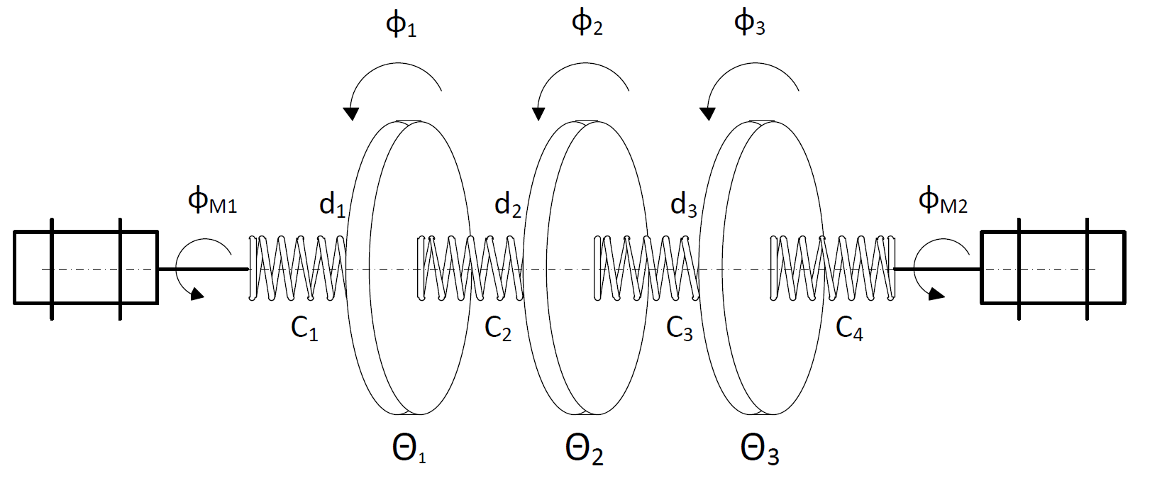
Three rotating discs are connected via springs and we denote their angles as \(\phi_1, \phi_2, \phi_3\). The two outermost discs are each connected to a stepper motor with additional springs. The stepper motor angles (\(\phi_{m,1}\) and \(\phi_{m,2}\) are used as inputs to the system. Relevant parameters of the system are the inertia \(\Theta\) of the three discs, the spring constants \(c\) as well as the damping factors \(d\).
The second degree ODE of this system can be written as follows:
\begin{align} \Theta_1 \ddot{\phi}_1 &= -c_1 \left(\phi_1 - \phi_{m,1} \right) -c_2 \left(\phi_1 - \phi_2 \right)- d_1 \dot{\phi}_1\\ \Theta_2 \ddot{\phi}_2 &= -c_2 \left(\phi_2 - \phi_{1} \right) -c_3 \left(\phi_2 - \phi_3 \right)- d_2 \dot{\phi}_2\\ \Theta_3 \ddot{\phi}_3 &= -c_3 \left(\phi_3 - \phi_2 \right) -c_4 \left(\phi_3 - \phi_{m,2} \right)- d_3 \dot{\phi}_3 \end{align}
The uncontrolled system, starting from a non-zero initial state will osciallate for an extended period of time, as shown below:

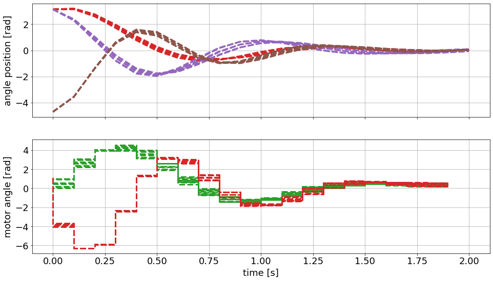
Later, we want to be able to use the motors efficiently to bring the oscillating masses to a rest. It will look something like this:
Creating the model#
As indicated above, the model block is essential for the application of do-mpc. In mathmatical terms the model is defined either as a continuous ordinary differential equation (ODE), a differential algebraic equation (DAE) or a discrete equation).
In the case of an DAE/ODE we write:
\begin{align} \frac{\partial x}{\partial t} &= f(x,u,z,p)\\ 0 &= g(x,u,z,p)\\ y &= h(x,u,z,p) \end{align}
We denote \(x\in \mathbb{R}^{n_x}\) as the states, \(u \in \mathbb{R}^{n_u}\) as the inputs, \(z\in \mathbb{R}^{n_z}\) the algebraic states and \(p \in \mathbb{R}^{n_p}\) as parameters.
We reformulate the second order ODEs above as the following first order ODEs, be introducing the following states:
\begin{align} x_1 &= \phi_1\\ x_2 &= \phi_2\\ x_3 &= \phi_3\\ x_4 &= \dot{\phi}_1\\ x_5 &= \dot{\phi}_2\\ x_6 &= \dot{\phi}_3\\ \end{align}
and derive the right-hand-side function \(f(x,u,z,p)\) as:
\begin{align} \dot{x}_1 &= x_4\\ \dot{x}_2 &= x_5\\ \dot{x}_3 &= x_6\\ \dot{x}_4 &= -\frac{c_1}{\Theta_1} \left(x_1 - u_1 \right) -\frac{c_2}{\Theta_1} \left(x1 - x_2 \right)- \frac{d_1}{\Theta_1} x_4\\ \dot{x}_5 &= -\frac{c_2}{\Theta_2} \left(x_2 - x_1 \right) -\frac{c_3}{\Theta_2} \left(x_2 - x_3 \right)- \frac{d_2}{\Theta_2} x_5\\ \dot{x}_6 &= -\frac{c_3}{\Theta_3} \left(x_3 - x_2 \right) -\frac{c_4}{\Theta_3} \left(x_4 - u_2 \right)- \frac{d_3}{\Theta_3} x_6\\ \end{align}
With this theoretical background we can start configuring the do-mpc model object.
First, we need to decide on the model type. For the given example, we are working with a continuous model.
[2]:
model_type = 'continuous' # either 'discrete' or 'continuous'
model = do_mpc.model.Model(model_type)
Model variables#
The next step is to define the model variables. It is important to define the variable type, name and optionally shape (default is scalar variable). The following types are available:
Long name |
short name |
Remark |
|---|---|---|
|
|
Required |
|
|
Required |
|
|
Optional |
|
|
Optional |
|
|
Optional |
[3]:
phi_1 = model.set_variable(var_type='_x', var_name='phi_1', shape=(1,1))
phi_2 = model.set_variable(var_type='_x', var_name='phi_2', shape=(1,1))
phi_3 = model.set_variable(var_type='_x', var_name='phi_3', shape=(1,1))
# Variables can also be vectors:
dphi = model.set_variable(var_type='_x', var_name='dphi', shape=(3,1))
# Two states for the desired (set) motor position:
phi_m_1_set = model.set_variable(var_type='_u', var_name='phi_m_1_set')
phi_m_2_set = model.set_variable(var_type='_u', var_name='phi_m_2_set')
# Two additional states for the true motor position:
phi_1_m = model.set_variable(var_type='_x', var_name='phi_1_m', shape=(1,1))
phi_2_m = model.set_variable(var_type='_x', var_name='phi_2_m', shape=(1,1))
Note that model.set_variable() returns the symbolic variable:
[4]:
print('phi_1={}, with phi_1.shape={}'.format(phi_1, phi_1.shape))
print('dphi={}, with dphi.shape={}'.format(dphi, dphi.shape))
phi_1=phi_1, with phi_1.shape=(1, 1)
dphi=[dphi_0, dphi_1, dphi_2], with dphi.shape=(3, 1)
Query variables#
If at any time you need to obtain the model variables, e.g. if you create the model in a different file than additional do-mpc modules, you might need to retrieve the defined variables. do-mpc facilitates this process with the Model properties x, u, z, p, tvp, y and aux:
[5]:
model.x
[5]:
<casadi.tools.structure3.ssymStruct at 0x7fa718a27d30>
The properties itself a structured symbolic variables, which hold the user-defined variables. These can be accessed with indices:
[6]:
model.x['phi_1']
[6]:
SX(phi_1)
Note that this is identical to the output of model.set_variable from above:
[7]:
bool(model.x['phi_1'] == phi_1)
[7]:
True
Further indices are possible in the case of variables with multiple elements:
[8]:
model.x['dphi',0]
[8]:
SX(dphi_0)
Note that you can use the following methods:
.keys().labels()
to get more information from the symbolic structures:
[9]:
model.x.keys()
[9]:
['phi_1', 'phi_2', 'phi_3', 'dphi', 'phi_1_m', 'phi_2_m']
[10]:
model.x.labels()
[10]:
['[phi_1,0]',
 '[phi_2,0]',
 '[phi_3,0]',
 '[dphi,0]',
 '[dphi,1]',
 '[dphi,2]',
 '[phi_1_m,0]',
 '[phi_2_m,0]']
Model parameters#
Next we define parameters. Known values can and should be hardcoded but with robust MPC in mind, we define uncertain parameters explictly. We assume that the inertia is such an uncertain parameter and hardcode the spring constant and friction coefficient.
[11]:
# As shown in the table above, we can use Long names or short names for the variable type.
Theta_1 = model.set_variable('parameter', 'Theta_1')
Theta_2 = model.set_variable('parameter', 'Theta_2')
Theta_3 = model.set_variable('parameter', 'Theta_3')

c = np.array([2.697,  2.66,  3.05, 2.86])*1e-3
d = np.array([6.78,  8.01,  8.82])*1e-5
Right-hand-side equation#
Finally, we set the right-hand-side of the model by calling model.set_rhs(var_name, expr) with the var_name from the state variables defined above and an expression in terms of \(x, u, z, p\).
[12]:
model.set_rhs('phi_1', dphi[0])
model.set_rhs('phi_2', dphi[1])
model.set_rhs('phi_3', dphi[2])
For the vector valued state dphi we need to concatenate symbolic expressions. We import the symbolic library CasADi:
[13]:
from casadi import *
[14]:
dphi_next = vertcat(
    -c[0]/Theta_1*(phi_1-phi_1_m)-c[1]/Theta_1*(phi_1-phi_2)-d[0]/Theta_1*dphi[0],
    -c[1]/Theta_2*(phi_2-phi_1)-c[2]/Theta_2*(phi_2-phi_3)-d[1]/Theta_2*dphi[1],
    -c[2]/Theta_3*(phi_3-phi_2)-c[3]/Theta_3*(phi_3-phi_2_m)-d[2]/Theta_3*dphi[2],
)

model.set_rhs('dphi', dphi_next)
[15]:
tau = 1e-2
model.set_rhs('phi_1_m', 1/tau*(phi_m_1_set - phi_1_m))
model.set_rhs('phi_2_m', 1/tau*(phi_m_2_set - phi_2_m))
The model setup is completed by calling model.setup():
[16]:
model.setup()
After calling model.setup() we cannot define further variables etc.
Configuring the MPC controller#
With the configured and setup model we can now create the optimizer for model predictive control (MPC). We start by creating the object (with the model as the only input)
[17]:
mpc = do_mpc.controller.MPC(model)
Optimizer parameters#
Next, we need to parametrize the optimizer. Please see the API documentation for optimizer.set_param() for a full description of available parameters and their meaning. Many parameters already have suggested default values. Most importantly, we need to set n_horizon and t_step. We also choose n_robust=1 for this example, which would default to 0.
Note that by default the continuous system is discretized with collocation.
[18]:
setup_mpc = {
    'n_horizon': 20,
    't_step': 0.1,
    'n_robust': 1,
    'store_full_solution': True,
}
mpc.set_param(**setup_mpc)
Objective function#
The MPC formulation is at its core an optimization problem for which we need to define an objective function:
We need to define the meyer term (mterm) and lagrange term (lterm). For the given example we set:
[19]:
mterm = phi_1**2 + phi_2**2 + phi_3**2
lterm = phi_1**2 + phi_2**2 + phi_3**2

mpc.set_objective(mterm=mterm, lterm=lterm)
Part of the objective function is also the penality for the control inputs. This penalty can often be used to smoothen the obtained optimal solution and is an important tuning parameter. We add a quadratic penalty on changes:
and automatically supply the solver with the previous solution of \(u_{k-1}\) for \(\Delta u_0\).
The user can set the tuning factor for these quadratic terms like this:
[20]:
mpc.set_rterm(
    phi_m_1_set=1e-2,
    phi_m_2_set=1e-2
)
where the keyword arguments refer to the previously defined input names. Note that in the notation above (\(\Delta u_k^T R \Delta u_k\)), this results in setting the diagonal elements of \(R\).
Constraints#
It is an important feature of MPC to be able to set constraints on inputs and states. In do-mpc these constraints are set like this:
[21]:
# Lower bounds on states:
mpc.bounds['lower','_x', 'phi_1'] = -2*np.pi
mpc.bounds['lower','_x', 'phi_2'] = -2*np.pi
mpc.bounds['lower','_x', 'phi_3'] = -2*np.pi
# Upper bounds on states
mpc.bounds['upper','_x', 'phi_1'] = 2*np.pi
mpc.bounds['upper','_x', 'phi_2'] = 2*np.pi
mpc.bounds['upper','_x', 'phi_3'] = 2*np.pi

# Lower bounds on inputs:
mpc.bounds['lower','_u', 'phi_m_1_set'] = -2*np.pi
mpc.bounds['lower','_u', 'phi_m_2_set'] = -2*np.pi
# Lower bounds on inputs:
mpc.bounds['upper','_u', 'phi_m_1_set'] = 2*np.pi
mpc.bounds['upper','_u', 'phi_m_2_set'] = 2*np.pi
Scaling#
Scaling is an important feature if the OCP is poorly conditioned, e.g. different states have significantly different magnitudes. In that case the unscaled problem might not lead to a (desired) solution. Scaling factors can be introduced for all states, inputs and algebraic variables and the objective is to scale them to roughly the same order of magnitude. For the given problem, this is not necessary but we briefly show the syntax (note that this step can also be skipped).
[22]:
mpc.scaling['_x', 'phi_1'] = 2
mpc.scaling['_x', 'phi_2'] = 2
mpc.scaling['_x', 'phi_3'] = 2
Uncertain Parameters#
An important feature of do-mpc is scenario based robust MPC. Instead of predicting and controlling a single future trajectory, we investigate multiple possible trajectories depending on different uncertain parameters. These parameters were previously defined in the model (the mass inertia). Now we must provide the optimizer with different possible scenarios.
This can be done in the following way:
[23]:
inertia_mass_1 = 2.25*1e-4*np.array([1., 0.9, 1.1])
inertia_mass_2 = 2.25*1e-4*np.array([1., 0.9, 1.1])
inertia_mass_3 = 2.25*1e-4*np.array([1.])

mpc.set_uncertainty_values(
    Theta_1 = inertia_mass_1,
    Theta_2 = inertia_mass_2,
    Theta_3 = inertia_mass_3
)
We provide a number of keyword arguments to the method optimizer.set_uncertain_parameter(). For each referenced parameter the value is a numpy.ndarray with a selection of possible values. The first value is the nominal case, where further values will lead to an increasing number of scenarios. Since we investigate each combination of possible parameters, the number of scenarios is growing rapidly. For our example, we are therefore only treating the inertia of mass 1 and 2 as uncertain and
supply only one possible value for the mass of inertia 3.
Setup#
The last step of configuring the optimizer is to call optimizer.setup, which finalizes the setup and creates the optimization problem. Only now can we use the optimizer to obtain the control input.
[24]:
mpc.setup()
Configuring the Simulator#
In many cases a developed control approach is first tested on a simulated system. do-mpc responds to this need with the do_mpc.simulator class. The simulator uses state-of-the-art DAE solvers, e.g. Sundials CVODE to solve the DAE equations defined in the supplied do_mpc.model. This will often be the same model as defined for the optimizer but it is also possible to use a more complex model of the same system.
In this section we demonstrate how to setup the simulator class for the given example. We initilize the class with the previously defined model:
[25]:
simulator = do_mpc.simulator.Simulator(model)
Simulator parameters#
Next, we need to parametrize the simulator. Please see the API documentation for simulator.set_param() for a full description of available parameters and their meaning. Many parameters already have suggested default values. Most importantly, we need to set t_step. We choose the same value as for the optimizer.
[26]:
# Instead of supplying a dict with the splat operator (**), as with the optimizer.set_param(),
# we can also use keywords (and call the method multiple times, if necessary):
simulator.set_param(t_step = 0.1)
Uncertain parameters#
In the model we have defined the inertia of the masses as parameters, for which we have chosen multiple scenarios in the optimizer. The simulator is now parametrized to simulate with the “true” values at each timestep. In the most general case, these values can change, which is why we need to supply a function that can be evaluted at each time to obtain the current values. do-mpc requires this function to have a specific return structure which we obtain first by calling:
[27]:
p_template = simulator.get_p_template()
This object is a CasADi structure:
[28]:
type(p_template)
[28]:
casadi.tools.structure3.DMStruct
which can be indexed with the following keys:
[29]:
p_template.keys()
[29]:
['default', 'Theta_1', 'Theta_2', 'Theta_3']
We need to now write a function which returns this structure with the desired numerical values. For our simple case:
[30]:
def p_fun(t_now):
    p_template['Theta_1'] = 2.25e-4
    p_template['Theta_2'] = 2.25e-4
    p_template['Theta_3'] = 2.25e-4
    return p_template
This function is now supplied to the simulator in the following way:
[31]:
simulator.set_p_fun(p_fun)
Setup#
Similarly to the optimizer we need to call simulator.setup() to finalize the setup of the simulator.
[32]:
simulator.setup()
Creating the control loop#
In theory, we could now also create an estimator but for this concise example we just assume direct state-feedback. This means we are now ready to setup and run the control loop. The control loop consists of running the optimizer with the current state (\(x_0\)) to obtain the current control input (\(u_0\)) and then running the simulator with the current control input (\(u_0\)) to obtain the next state.
As discussed before, we setup a controller for regulating a triple-mass-spring system. To show some interesting control action we choose an arbitrary initial state \(x_0\neq 0\):
[33]:
x0 = np.pi*np.array([1, 1, -1.5, 1, -1, 1, 0, 0]).reshape(-1,1)
and use the x0 property to set the initial state.
[34]:
simulator.x0 = x0
mpc.x0 = x0
While we are able to set just a regular numpy array, this populates the state structure which was inherited from the model:
[35]:
mpc.x0
[35]:
<casadi.tools.structure3.DMStruct at 0x7fa71b5ee390>
We can thus easily obtain the value of particular states by calling:
[36]:
mpc.x0['phi_1']
[36]:
DM(3.14159)
Note that the properties x0 (as well as u0, z0 and t0) always display the values of the current variables in the class.
To set the initial guess of the MPC optimization problem we call:
[37]:
mpc.set_initial_guess()
The chosen initial guess is based on x0, z0 and u0 which are set for each element of the MPC sequence.
Setting up the Graphic#
To investigate the controller performance AND the MPC predictions, we are using the do-mpc graphics module. This versatile tool allows us to conveniently configure a user-defined plot based on Matplotlib and visualize the results stored in the mpc.data, simulator.data (and if applicable estimator.data) objects.
We start by importing matplotlib:
[38]:
import matplotlib.pyplot as plt
import matplotlib as mpl
# Customizing Matplotlib:
mpl.rcParams['font.size'] = 18
mpl.rcParams['lines.linewidth'] = 3
mpl.rcParams['axes.grid'] = True
And initializing the graphics module with the data object of interest. In this particular example, we want to visualize both the mpc.data as well as the simulator.data.
[39]:
mpc_graphics = do_mpc.graphics.Graphics(mpc.data)
sim_graphics = do_mpc.graphics.Graphics(simulator.data)
Next, we create a figure and obtain its axis object. Matplotlib offers multiple alternative ways to obtain an axis object, e.g. subplots, subplot2grid, or simply gca. We use subplots:
[40]:
%%capture
# We just want to create the plot and not show it right now. This "inline magic" supresses the output.
fig, ax = plt.subplots(2, sharex=True, figsize=(16,9))
fig.align_ylabels()
Most important API element for setting up the graphics module is graphics.add_line, which mimics the API of model.add_variable, except that we also need to pass an axis.
We want to show both the simulator and MPC results on the same axis, which is why we configure both of them identically:
[41]:
%%capture
for g in [sim_graphics, mpc_graphics]:
    # Plot the angle positions (phi_1, phi_2, phi_2) on the first axis:
    g.add_line(var_type='_x', var_name='phi_1', axis=ax[0])
    g.add_line(var_type='_x', var_name='phi_2', axis=ax[0])
    g.add_line(var_type='_x', var_name='phi_3', axis=ax[0])

    # Plot the set motor positions (phi_m_1_set, phi_m_2_set) on the second axis:
    g.add_line(var_type='_u', var_name='phi_m_1_set', axis=ax[1])
    g.add_line(var_type='_u', var_name='phi_m_2_set', axis=ax[1])


ax[0].set_ylabel('angle position [rad]')
ax[1].set_ylabel('motor angle [rad]')
ax[1].set_xlabel('time [s]')
Running the simulator#
We start investigating the do-mpc simulator and the graphics package by simulating the autonomous system without control inputs (\(u = 0\)). This can be done as follows:
[42]:
u0 = np.zeros((2,1))
for i in range(200):
    simulator.make_step(u0)
We can visualize the resulting trajectory with the pre-defined graphic:
[43]:
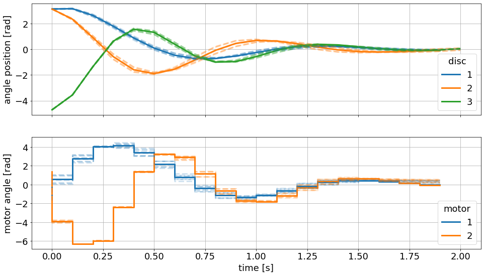
sim_graphics.plot_results()
# Reset the limits on all axes in graphic to show the data.
sim_graphics.reset_axes()
# Show the figure:
fig
[43]:
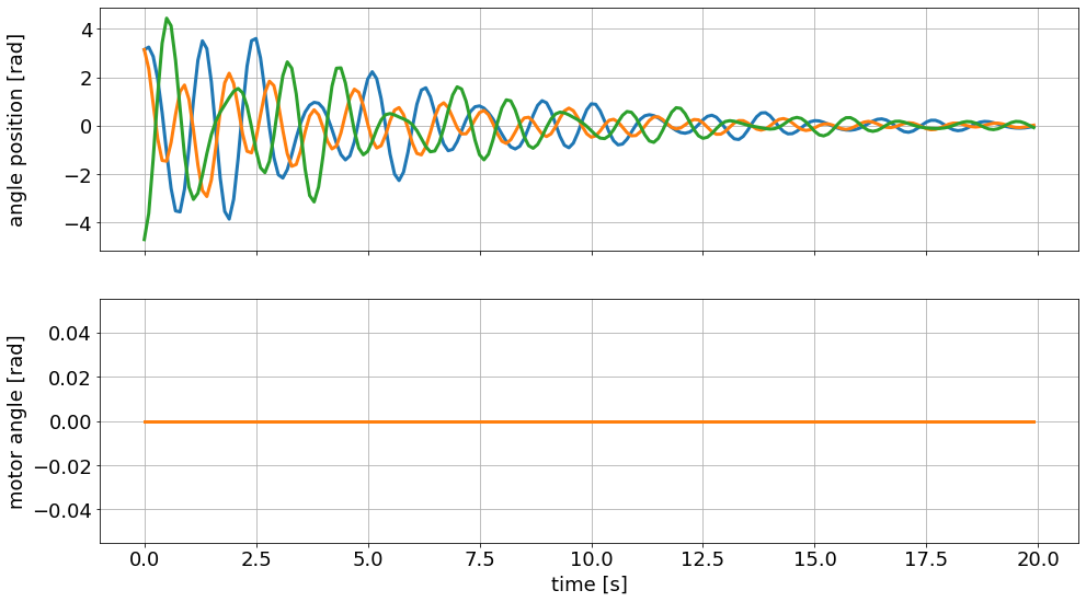
As desired, the motor angle (input) is constant at zero and the oscillating masses slowly come to a rest. Our control goal is to significantly shorten the time until the discs are stationary.
Remember the animation you saw above, of the uncontrolled system? This is where the data came from.
Running the optimizer#
To obtain the current control input we call optimizer.make_step(x0) with the current state (\(x_0\)):
[44]:
u0 = mpc.make_step(x0)
******************************************************************************
This program contains Ipopt, a library for large-scale nonlinear optimization.
 Ipopt is released as open source code under the Eclipse Public License (EPL).
         For more information visit http://projects.coin-or.org/Ipopt
******************************************************************************

This is Ipopt version 3.12.3, running with linear solver mumps.
NOTE: Other linear solvers might be more efficient (see Ipopt documentation).

Number of nonzeros in equality constraint Jacobian...:    19448
Number of nonzeros in inequality constraint Jacobian.:        0
Number of nonzeros in Lagrangian Hessian.............:     1229

Total number of variables............................:     6408
                     variables with only lower bounds:        0
                variables with lower and upper bounds:     2435
                     variables with only upper bounds:        0
Total number of equality constraints.................:     5768
Total number of inequality constraints...............:        0
        inequality constraints with only lower bounds:        0
   inequality constraints with lower and upper bounds:        0
        inequality constraints with only upper bounds:        0

iter    objective    inf_pr   inf_du lg(mu)  ||d||  lg(rg) alpha_du alpha_pr  ls
   0  8.8086219e+02 1.65e+01 1.07e-01  -1.0 0.00e+00    -  0.00e+00 0.00e+00   0
   1  2.8794996e+02 2.32e+00 1.68e+00  -1.0 1.38e+01  -4.0 2.82e-01 8.60e-01f  1
   2  2.0017562e+02 1.87e-14 3.95e+00  -1.0 3.56e+00  -4.5 1.96e-01 1.00e+00f  1
   3  1.6039802e+02 1.48e-14 3.82e-01  -1.0 3.43e+00  -5.0 5.14e-01 1.00e+00f  1
   4  1.3046012e+02 2.04e-14 7.36e-02  -1.0 2.94e+00  -5.4 7.75e-01 1.00e+00f  1
   5  1.1452477e+02 2.04e-14 1.94e-02  -1.7 2.62e+00  -5.9 8.44e-01 1.00e+00f  1
   6  1.1247422e+02 1.87e-14 7.23e-03  -2.5 9.17e-01  -6.4 8.27e-01 1.00e+00f  1
   7  1.1235000e+02 1.69e-14 4.88e-08  -2.5 3.56e-01  -6.9 1.00e+00 1.00e+00f  1
   8  1.1230585e+02 1.87e-14 8.91e-09  -3.8 1.95e-01  -7.3 1.00e+00 1.00e+00f  1
   9  1.1229857e+02 1.83e-14 8.02e-10  -5.7 5.26e-02  -7.8 1.00e+00 1.00e+00f  1
iter    objective    inf_pr   inf_du lg(mu)  ||d||  lg(rg) alpha_du alpha_pr  ls
  10  1.1229833e+02 1.51e-14 6.08e-09  -5.7 1.20e+00  -8.3 1.00e+00 1.00e+00f  1
  11  1.1229831e+02 1.69e-14 3.25e-13  -8.6 1.92e-04  -8.8 1.00e+00 1.00e+00f  1

Number of Iterations....: 11

                                   (scaled)                 (unscaled)
Objective...............:   1.1229831239969913e+02    1.1229831239969913e+02
Dual infeasibility......:   3.2479227640713759e-13    3.2479227640713759e-13
Constraint violation....:   1.6875389974302379e-14    1.6875389974302379e-14
Complementarity.........:   4.2481089749952700e-09    4.2481089749952700e-09
Overall NLP error.......:   4.2481089749952700e-09    4.2481089749952700e-09


Number of objective function evaluations             = 12
Number of objective gradient evaluations             = 12
Number of equality constraint evaluations            = 12
Number of inequality constraint evaluations          = 0
Number of equality constraint Jacobian evaluations   = 12
Number of inequality constraint Jacobian evaluations = 0
Number of Lagrangian Hessian evaluations             = 11
Total CPU secs in IPOPT (w/o function evaluations)   =      0.239
Total CPU secs in NLP function evaluations           =      0.006

EXIT: Optimal Solution Found.
           S  :   t_proc      (avg)   t_wall      (avg)    n_eval
       nlp_f  | 149.00us ( 12.42us) 145.00us ( 12.08us)        12
       nlp_g  |   2.16ms (180.17us)   1.83ms (152.33us)        12
    nlp_grad  | 377.00us (377.00us) 377.00us (377.00us)         1
  nlp_grad_f  | 504.00us ( 38.77us) 525.00us ( 40.38us)        13
  nlp_hess_l  | 138.00us ( 12.55us) 137.00us ( 12.45us)        11
   nlp_jac_g  |   3.27ms (251.31us)   3.26ms (251.00us)        13
       total  | 257.31ms (257.31ms) 256.06ms (256.06ms)         1
Note that we obtained the output from IPOPT regarding the given optimal control problem (OCP). Most importantly we obtained Optimal Solution Found.
We can also visualize the predicted trajectories with the configure graphics instance. First we clear the existing lines from the simulator by calling:
[45]:
sim_graphics.clear()
And finally, we can call plot_predictions to obtain:
[46]:
mpc_graphics.plot_predictions()
mpc_graphics.reset_axes()
# Show the figure:
fig
[46]:
We are seeing the predicted trajectories for the states and the optimal control inputs. Note that we are seeing different scenarios for the configured uncertain inertia of the three masses.
We can also see that the solution is considering the defined upper and lower bounds. This is especially true for the inputs.
Changing the line appearance#
Before we continue, we should probably improve the visualization a bit. We can easily obtain all line objects from the graphics module by using the result_lines and pred_lines properties:
[47]:
mpc_graphics.pred_lines
[47]:
<do_mpc.tools.structure.Structure at 0x7fa71b5ee860>
We obtain a structure that can be queried conveniently as follows:
[48]:
mpc_graphics.pred_lines['_x', 'phi_1']
[48]:
[<matplotlib.lines.Line2D at 0x7fa71c445828>,
 <matplotlib.lines.Line2D at 0x7fa71c6e7898>,
 <matplotlib.lines.Line2D at 0x7fa71c6e7978>,
 <matplotlib.lines.Line2D at 0x7fa71c7023c8>,
 <matplotlib.lines.Line2D at 0x7fa71c7022b0>,
 <matplotlib.lines.Line2D at 0x7fa71c702630>,
 <matplotlib.lines.Line2D at 0x7fa71c702978>,
 <matplotlib.lines.Line2D at 0x7fa71c702d30>,
 <matplotlib.lines.Line2D at 0x7fa71c702c88>]
We obtain all lines for our first state. To change the color we can simply:
[49]:
# Change the color for the three states:
for line_i in mpc_graphics.pred_lines['_x', 'phi_1']: line_i.set_color('#1f77b4') # blue
for line_i in mpc_graphics.pred_lines['_x', 'phi_2']: line_i.set_color('#ff7f0e') # orange
for line_i in mpc_graphics.pred_lines['_x', 'phi_3']: line_i.set_color('#2ca02c') # green
# Change the color for the two inputs:
for line_i in mpc_graphics.pred_lines['_u', 'phi_m_1_set']: line_i.set_color('#1f77b4')
for line_i in mpc_graphics.pred_lines['_u', 'phi_m_2_set']: line_i.set_color('#ff7f0e')

# Make all predictions transparent:
for line_i in mpc_graphics.pred_lines.full: line_i.set_alpha(0.2)
Note that we can work in the same way with the result_lines property. For example, we can use it to create a legend:
[50]:
# Get line objects (note sum of lists creates a concatenated list)
lines = sim_graphics.result_lines['_x', 'phi_1']+sim_graphics.result_lines['_x', 'phi_2']+sim_graphics.result_lines['_x', 'phi_3']

ax[0].legend(lines,'123',title='disc')

# also set legend for second subplot:
lines = sim_graphics.result_lines['_u', 'phi_m_1_set']+sim_graphics.result_lines['_u', 'phi_m_2_set']
ax[1].legend(lines,'12',title='motor')
[50]:
<matplotlib.legend.Legend at 0x7fa71c712eb8>
Running the control loop#
Finally, we are now able to run the control loop as discussed above. We obtain the input from the optimizer and then run the simulator.
To make sure we start fresh, we erase the history and set the initial state for the simulator:
[51]:
simulator.reset_history()
simulator.x0 = x0
mpc.reset_history()
This is the main-loop. We run 20 steps, whic is identical to the prediction horizon. Note that we use “capture” again, to supress the output from IPOPT.
It is usually suggested to display the output as it contains important information about the state of the solver.
[52]:
%%capture
for i in range(20):
    u0 = mpc.make_step(x0)
    x0 = simulator.make_step(u0)
We can now plot the previously shown prediction from time \(t=0\), as well as the closed-loop trajectory from the simulator:
[53]:
# Plot predictions from t=0
mpc_graphics.plot_predictions(t_ind=0)
# Plot results until current time
sim_graphics.plot_results()
sim_graphics.reset_axes()
fig
[53]:
The simulated trajectory with the nominal value of the parameters follows almost exactly the nominal open-loop predictions. The simulted trajectory is bounded from above and below by further uncertain scenarios.
Data processing#
Saving and retrieving results#
do-mpc results can be stored and retrieved with the methods save_results and load_results from the do_mpc.data module. We start by importing these methods:
[55]:
from do_mpc.data import save_results, load_results
The method save_results is passed a list of the do-mpc objects that we want to store. In our case, the optimizer and simulator are available and configured.
Note that by default results are stored in the subfolder results under the name results.pkl. Both can be changed and the folder is created if it doesn’t exist already.
[56]:
save_results([mpc, simulator])
We investigate the content of the newly created folder:
[57]:
!ls ./results/
results.pkl
Automatically, the save_results call will check if a file with the given name already exists. To avoid overwriting, the method prepends an index. If we save again, the folder contains:
[58]:
save_results([mpc, simulator])
!ls ./results/
001_results.pkl results.pkl
The pickled results can be loaded manually by writing:
with open(file_name, 'rb') as f:
    results = pickle.load(f)
or by calling load_results with the appropriate file_name (and path). load_results contains simply the code above for more convenience.
[59]:
results = load_results('./results/results.pkl')
The obtained results is a dictionary with the data objects from the passed do-mpc modules. Such that: results['optimizer'] and optimizer.data contain the same information (similarly for simulator and, if applicable, estimator).
Working with data objects#
The do_mpc.data.Data objects also hold some very useful properties that you should know about. Most importantly, we can query them with indices, such as:
[60]:
results['mpc']
[60]:
<do_mpc.data.MPCData at 0x117c4df50>
[61]:
x = results['mpc']['_x']
x.shape
[61]:
(20, 8)
As expected, we have 20 elements (we ran the loop for 20 steps) and 8 states. Further indices allow to get selected states:
[62]:
phi_1 = results['mpc']['_x','phi_1']

phi_1.shape
[62]:
(20, 1)
For vector-valued states we can even query:
[63]:
dphi_1 = results['mpc']['_x','dphi', 0]

dphi_1.shape
[63]:
(20, 1)
Of course, we could also query inputs etc.
Furthermore, we can easily retrieve the predicted trajectories with the prediction method. The syntax is slightly different: The first argument is a tuple that mimics the indices shown above. The second index is the time instance. With the following call we obtain the prediction of phi_1 at time 0:
[64]:
phi_1_pred = results['mpc'].prediction(('_x','phi_1'), t_ind=0)

phi_1_pred.shape
[64]:
(1, 21, 9)
The first dimension shows that this state is a scalar, the second dimension shows the horizon and the third dimension refers to the nine uncertain scenarios that were investigated.
Animating results#
Animating MPC results, to compare prediction and closed-loop trajectories, allows for a very meaningful investigation of the obtained results.
do-mpc significantly facilitates this process while working hand in hand with Matplotlib for full customizability. Obtaining publication ready animations is as easy as writing the following short blocks of code:
[66]:
from matplotlib.animation import FuncAnimation, FFMpegWriter, ImageMagickWriter

def update(t_ind):
    sim_graphics.plot_results(t_ind)
    mpc_graphics.plot_predictions(t_ind)
    mpc_graphics.reset_axes()
The graphics module can also be used without restrictions with loaded do-mpc data. This allows for convenient data post-processing, e.g. in a Jupyter Notebook. We simply would have to initiate the graphics module with the loaded results from above.
[69]:
anim = FuncAnimation(fig, update, frames=20, repeat=False)
gif_writer = ImageMagickWriter(fps=3)
anim.save('anim.gif', writer=gif_writer)
Below we showcase the resulting gif file (not in real-time): 
Thank you, for following through this short example on how to use do-mpc. We hope you find the tool and this documentation useful.
We suggest that you have a look at the API documentation for further details on the presented modules, methods and functions.
We also want to emphasize that we skipped over many details, further functions etc. in this introduction. Please have a look at our more complex examples to get a better impression of the possibilities with do-mpc.